Show the code
pacman::p_load(tidymodels, readr, earth, ggthemr, vip, glue)
ggthemr(palette = "fresh", layout = "scientific", spacing = 3)This project aims to predict crop yield using Multivariate Adaptive Regression Splines (MARS) implemented with the earth package by Stephen Milborrow. In this project we will walk through data loading, some exploratory data analysis, preprocessing, model specification, tuning, and performance evaluation.
We’ll load tidymodels, ggthemr, earth and vip packages using pacman’s p_load() function.
pacman::p_load(tidymodels, readr, earth, ggthemr, vip, glue)
ggthemr(palette = "fresh", layout = "scientific", spacing = 3)Here, we load the dataset and clean up column names for easier reference. Then, we review the data structure and conduct an initial exploration of its properties. The data was gotten from kaggle data repository. The dataset contains agricultural data for 1,000,000 samples aimed at predicting crop yield (in tons per hectare) based on various factors. The features of the data are:
crop_yield <- read_csv("data/crop_yield.csv") |>
  janitor::clean_names()
To get a detailed summary of the data, we use skimr()
skimr::skim_without_charts(crop_yield)| Name | crop_yield |
| Number of rows | 1000000 |
| Number of columns | 10 |
| _______________________ | |
| Column type frequency: | |
| character | 4 |
| logical | 2 |
| numeric | 4 |
| ________________________ | |
| Group variables | None |
Variable type: character
| skim_variable | n_missing | complete_rate | min | max | empty | n_unique | whitespace |
|---|---|---|---|---|---|---|---|
| region | 0 | 1 | 4 | 5 | 0 | 4 | 0 |
| soil_type | 0 | 1 | 4 | 6 | 0 | 6 | 0 |
| crop | 0 | 1 | 4 | 7 | 0 | 6 | 0 |
| weather_condition | 0 | 1 | 5 | 6 | 0 | 3 | 0 |
Variable type: logical
| skim_variable | n_missing | complete_rate | mean | count |
|---|---|---|---|---|
| fertilizer_used | 0 | 1 | 0.5 | FAL: 500060, TRU: 499940 |
| irrigation_used | 0 | 1 | 0.5 | FAL: 500509, TRU: 499491 |
Variable type: numeric
| skim_variable | n_missing | complete_rate | mean | sd | p0 | p25 | p50 | p75 | p100 |
|---|---|---|---|---|---|---|---|---|---|
| rainfall_mm | 0 | 1 | 549.98 | 259.85 | 100.00 | 324.89 | 550.12 | 774.74 | 1000.00 |
| temperature_celsius | 0 | 1 | 27.50 | 7.22 | 15.00 | 21.25 | 27.51 | 33.75 | 40.00 |
| days_to_harvest | 0 | 1 | 104.50 | 25.95 | 60.00 | 82.00 | 104.00 | 127.00 | 149.00 |
| yield_tons_per_hectare | 0 | 1 | 4.65 | 1.70 | -1.15 | 3.42 | 4.65 | 5.88 | 9.96 |
The result from Table 1 shows the data is complete.
To ensure proper model performance, we change character data types into categorical data types (factors in R).
Categorical variables are more suited to analysis than character as they are mapped to numerical values. There’re more reasons, but the one given is enough.
crop_yield <- crop_yield |>
  mutate(
    across(where(is.character), factor)
)Let’s explore some of the relationship between the target variables and the predictors.
subtitle <- glue(
  "The {length(unique(crop_yield$crop))} crops are distributed uniformly across the different regions"
)

ggplot(
  data = crop_yield,
  aes(region, y = after_stat(count), fill = crop)
) +
  geom_bar(position = "dodge") +
  labs(
    title = "Frequency of crop types across regions",
    subtitle = subtitle
  ) +
  theme(
    axis.ticks.x = element_blank()
  )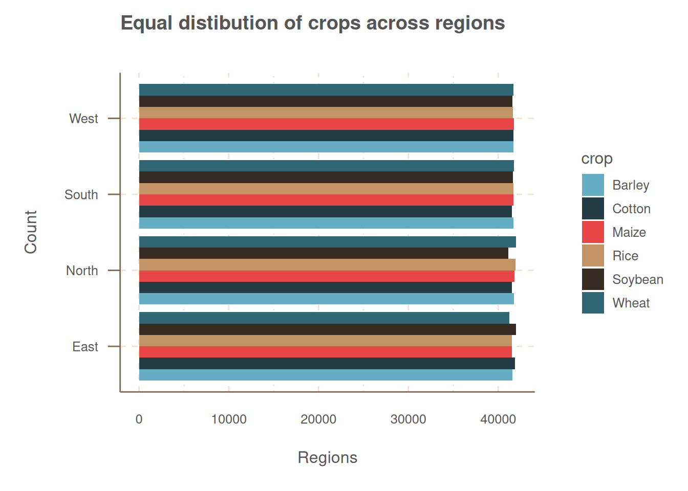
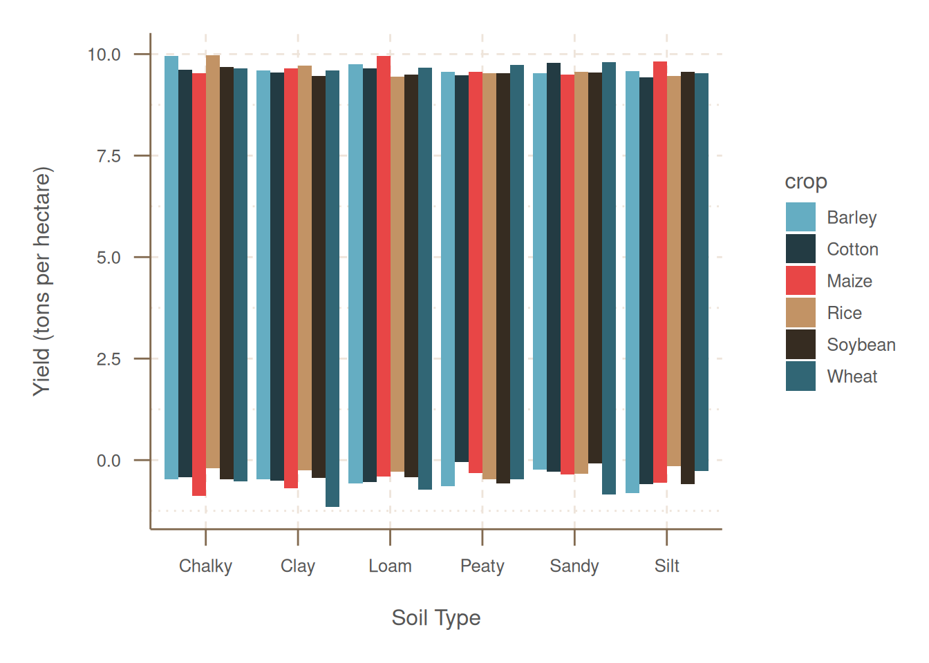
Figure 1 shows that crops are uniformly distributed across the regions. The same can also be said for the yield across across the different soil types Figure 2.
ggplot(crop_yield, aes(soil_type, yield_tons_per_hectare,  fill = crop)) +
  geom_violin(
    position = position_dodge(width = 0.8),
    alpha = .8
  ) +
  labs(
    x = "Soil Type",
    y = "Yield (tons per hectare)"
  )
crop_yield |>
  ggplot(aes(yield_tons_per_hectare)) +
  geom_histogram() +
  labs(
    x = "Yield (tons per hectare)",
    y = "Count",
    title = "Target variable (Yield) distribution"
  ) +
  theme(
    plot.title = element_text(hjust = .5)
  )
`stat_bin()` using `bins = 30`. Pick better value `binwidth`.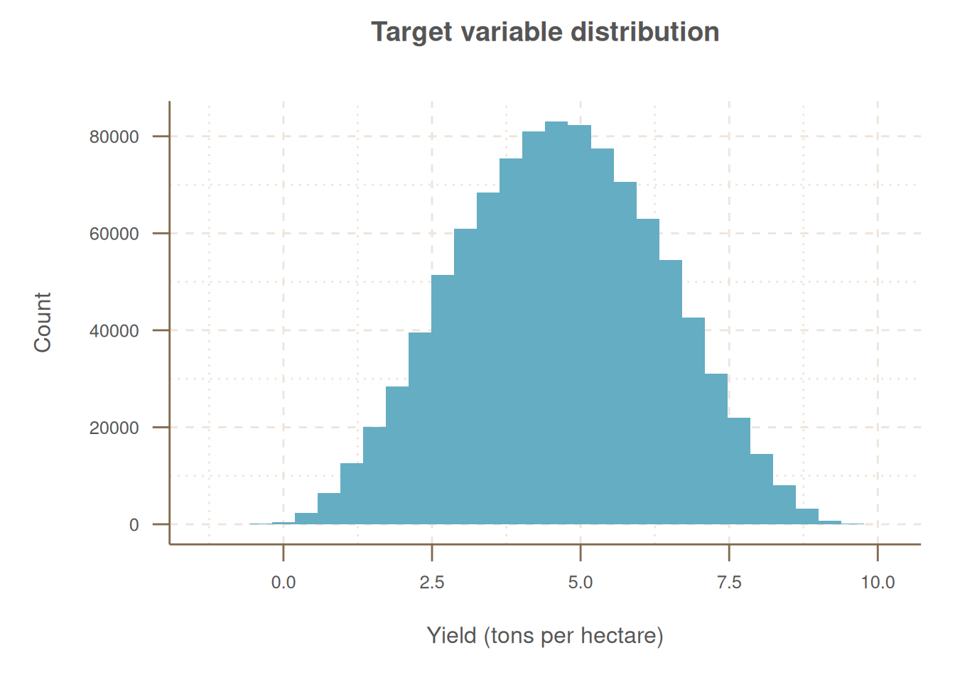
The data will be split into two part. The first which is the training data will be 70 % of all data and the second, the testing data will be 30 % of all the data.
set.seed(1012)
crop_yield_split <- crop_yield |> initial_split(prop = c(.7))

crop_train <- training(crop_yield_split)
crop_test <- testing(crop_yield_split)
Given the size of the training data, 700000 rows, 5 folds cross validation data will be used for evaluating the models.
crop_fold <- vfold_cv(crop_train, v = 5)As stated in the start, we’ll be using the multivariate adaptive regression splines (MARS) model. Two parameters, the prod_degree, which captures the maximum degree of interactions, and the num_terms which determine the maximum number of features to retain in the final model will be tuned.
mars_spec <- mars(
  prod_degree = tune(),
  num_terms = tune()
) |>
  set_mode("regression") |>
set_engine("earth")MARS model generally require less preprocessing except creating dummy variables. Feature engineering methods and steps such as feature decorrelation and data transformation are not needed but might help the model.
mars_rec <- recipe(
  yield_tons_per_hectare ~ .,
  data = crop_train
  ) |>
  step_mutate(across(where(is_logical), \(x) factor(x))) |>
  step_pca(all_numeric_predictors()) |>
  step_dummy(all_factor_predictors())
The preprocessed data can be seen in Table 2
mars_rec |>
  prep() |>
  juice() |>
  head(n = 50) |>
knitr::kable()| yield_tons_per_hectare | PC1 | PC2 | PC3 | region_North | region_South | region_West | soil_type_Clay | soil_type_Loam | soil_type_Peaty | soil_type_Sandy | soil_type_Silt | crop_Cotton | crop_Maize | crop_Rice | crop_Soybean | crop_Wheat | fertilizer_used_TRUE. | irrigation_used_TRUE. | weather_condition_Rainy | weather_condition_Sunny |
|---|---|---|---|---|---|---|---|---|---|---|---|---|---|---|---|---|---|---|---|---|
| 3.400731 | -443.5131 | -3.2544271 | 6.5953117 | 0 | 0 | 0 | 0 | 0 | 0 | 1 | 0 | 0 | 0 | 0 | 0 | 0 | 0 | 0 | 0 | 1 |
| 5.751228 | -413.4660 | 38.4651334 | -4.7839110 | 0 | 1 | 0 | 1 | 0 | 0 | 0 | 0 | 0 | 0 | 0 | 1 | 0 | 1 | 1 | 0 | 1 |
| 1.008976 | -168.7606 | 87.5538465 | -6.0975899 | 0 | 1 | 0 | 0 | 0 | 0 | 0 | 1 | 0 | 0 | 0 | 1 | 0 | 0 | 0 | 0 | 1 |
| 3.717387 | -394.7569 | 45.5903100 | 10.3686348 | 1 | 0 | 0 | 0 | 0 | 1 | 0 | 0 | 0 | 0 | 0 | 0 | 0 | 0 | 1 | 1 | 0 |
| 5.396987 | -720.9266 | -46.7551966 | 15.2481557 | 0 | 1 | 0 | 0 | 0 | 0 | 1 | 0 | 0 | 1 | 0 | 0 | 0 | 1 | 0 | 0 | 1 |
| 5.451859 | -711.6603 | -41.3647498 | 19.2116423 | 0 | 1 | 0 | 0 | 1 | 0 | 0 | 0 | 0 | 1 | 0 | 0 | 0 | 1 | 0 | 1 | 0 |
| 3.684737 | -495.8147 | 13.1038455 | 16.1939490 | 0 | 0 | 1 | 0 | 0 | 0 | 1 | 0 | 0 | 0 | 0 | 0 | 0 | 0 | 1 | 1 | 0 |
| 3.023139 | -686.8627 | 25.5219354 | -11.4658760 | 0 | 0 | 1 | 0 | 0 | 0 | 0 | 0 | 0 | 0 | 0 | 1 | 0 | 0 | 0 | 1 | 0 |
| 1.723296 | -323.3785 | 36.9915343 | 8.6552575 | 1 | 0 | 0 | 0 | 0 | 0 | 1 | 0 | 0 | 0 | 1 | 0 | 0 | 0 | 0 | 0 | 0 |
| 4.634474 | -950.9416 | -69.5868045 | -2.8519015 | 0 | 0 | 1 | 0 | 0 | 0 | 1 | 0 | 0 | 0 | 0 | 1 | 0 | 0 | 0 | 1 | 0 |
| 1.747024 | -277.6119 | 94.8666909 | 3.3706059 | 0 | 1 | 0 | 0 | 1 | 0 | 0 | 0 | 1 | 0 | 0 | 0 | 0 | 0 | 0 | 0 | 1 |
| 5.838846 | -744.2276 | 28.8373686 | -16.1826853 | 1 | 0 | 0 | 1 | 0 | 0 | 0 | 0 | 0 | 1 | 0 | 0 | 0 | 1 | 0 | 1 | 0 |
| 6.912032 | -872.8384 | -41.7072329 | 6.8584246 | 0 | 1 | 0 | 0 | 1 | 0 | 0 | 0 | 0 | 0 | 0 | 0 | 0 | 1 | 0 | 1 | 0 |
| 3.580292 | -240.0413 | 58.2084201 | 1.9630820 | 1 | 0 | 0 | 0 | 1 | 0 | 0 | 0 | 0 | 0 | 0 | 0 | 1 | 1 | 0 | 1 | 0 |
| 5.970243 | -810.7648 | -28.6007998 | -7.7296912 | 0 | 1 | 0 | 1 | 0 | 0 | 0 | 0 | 0 | 1 | 0 | 0 | 0 | 0 | 1 | 0 | 0 |
| 5.521300 | -962.8168 | -61.4827331 | -4.4806095 | 0 | 1 | 0 | 0 | 1 | 0 | 0 | 0 | 0 | 0 | 0 | 0 | 1 | 0 | 1 | 0 | 1 |
| 8.264468 | -1005.1906 | -16.2531142 | -17.9959450 | 0 | 0 | 0 | 0 | 0 | 0 | 0 | 0 | 0 | 0 | 1 | 0 | 0 | 1 | 1 | 1 | 0 |
| 2.617062 | -261.3142 | 37.6294917 | 8.8437005 | 1 | 0 | 0 | 1 | 0 | 0 | 0 | 0 | 0 | 0 | 0 | 0 | 0 | 0 | 1 | 0 | 1 |
| 1.293327 | -221.4408 | 86.5704468 | -0.1552813 | 0 | 1 | 0 | 0 | 0 | 0 | 0 | 1 | 0 | 0 | 0 | 0 | 1 | 0 | 0 | 0 | 0 |
| 4.575414 | -554.1366 | 0.8347687 | 16.8366677 | 0 | 1 | 0 | 0 | 0 | 0 | 1 | 0 | 0 | 1 | 0 | 0 | 0 | 0 | 1 | 0 | 1 |
| 4.135580 | -192.6099 | 49.8051290 | 19.8209766 | 0 | 1 | 0 | 0 | 0 | 0 | 0 | 0 | 0 | 1 | 0 | 0 | 0 | 1 | 1 | 0 | 0 |
| 3.583365 | -401.2845 | 52.4689066 | -11.4656548 | 0 | 1 | 0 | 0 | 0 | 0 | 0 | 0 | 1 | 0 | 0 | 0 | 0 | 1 | 0 | 0 | 0 |
| 3.496146 | -671.5287 | -23.9025896 | 12.6958034 | 0 | 0 | 1 | 1 | 0 | 0 | 0 | 0 | 0 | 1 | 0 | 0 | 0 | 0 | 0 | 0 | 1 |
| 2.024070 | -385.8237 | 75.9651378 | 5.4313029 | 1 | 0 | 0 | 0 | 0 | 0 | 0 | 1 | 0 | 1 | 0 | 0 | 0 | 0 | 0 | 1 | 0 |
| 4.470276 | -556.4865 | -3.4993558 | 7.6085121 | 0 | 1 | 0 | 1 | 0 | 0 | 0 | 0 | 0 | 0 | 0 | 0 | 1 | 1 | 0 | 0 | 0 |
| 2.636910 | -309.2241 | 94.1466605 | -15.8569091 | 0 | 0 | 1 | 0 | 0 | 0 | 0 | 0 | 0 | 0 | 1 | 0 | 0 | 1 | 0 | 0 | 1 |
| 4.778564 | -734.4747 | -20.6729247 | -3.2105890 | 1 | 0 | 0 | 0 | 1 | 0 | 0 | 0 | 0 | 1 | 0 | 0 | 0 | 0 | 1 | 0 | 0 |
| 4.740436 | -643.3828 | 50.6757693 | -3.2353822 | 1 | 0 | 0 | 0 | 0 | 0 | 1 | 0 | 0 | 0 | 1 | 0 | 0 | 0 | 1 | 0 | 1 |
| 4.247667 | -399.0755 | 71.8376503 | 0.6495655 | 0 | 0 | 1 | 0 | 0 | 0 | 1 | 0 | 1 | 0 | 0 | 0 | 0 | 1 | 0 | 0 | 0 |
| 3.152931 | -598.4676 | 24.8970443 | -2.6472120 | 1 | 0 | 0 | 0 | 0 | 1 | 0 | 0 | 0 | 0 | 1 | 0 | 0 | 0 | 0 | 1 | 0 |
| 6.976502 | -814.5275 | 16.4940887 | -1.5522390 | 0 | 0 | 0 | 0 | 0 | 0 | 0 | 1 | 0 | 0 | 0 | 0 | 1 | 1 | 1 | 0 | 1 |
| 4.418112 | -522.9164 | 32.8871108 | -2.2873263 | 0 | 1 | 0 | 0 | 1 | 0 | 0 | 0 | 0 | 0 | 1 | 0 | 0 | 1 | 0 | 1 | 0 |
| 2.083175 | -126.8781 | 103.7691760 | -9.9791434 | 0 | 0 | 0 | 0 | 0 | 0 | 0 | 1 | 0 | 0 | 0 | 0 | 1 | 0 | 1 | 1 | 0 |
| 4.663298 | -532.6092 | 17.1725916 | 14.2671621 | 0 | 1 | 0 | 0 | 1 | 0 | 0 | 0 | 0 | 0 | 0 | 0 | 1 | 0 | 1 | 1 | 0 |
| 4.975227 | -686.0732 | 25.6109428 | -1.5719943 | 0 | 0 | 0 | 0 | 1 | 0 | 0 | 0 | 0 | 1 | 0 | 0 | 0 | 0 | 0 | 1 | 0 |
| 3.630072 | -415.7840 | 2.4882849 | 18.0693031 | 0 | 0 | 1 | 0 | 0 | 0 | 0 | 0 | 0 | 0 | 0 | 1 | 0 | 1 | 0 | 1 | 0 |
| 6.452334 | -997.9162 | -74.9602323 | -7.6363843 | 0 | 1 | 0 | 0 | 0 | 0 | 0 | 1 | 0 | 0 | 0 | 0 | 0 | 1 | 0 | 0 | 0 |
| 6.011272 | -818.8715 | -25.8789875 | -13.3425221 | 0 | 0 | 0 | 0 | 0 | 0 | 1 | 0 | 1 | 0 | 0 | 0 | 0 | 1 | 0 | 0 | 0 |
| 4.366196 | -839.1552 | -26.0351393 | 1.6664309 | 0 | 1 | 0 | 0 | 0 | 0 | 0 | 0 | 0 | 0 | 0 | 0 | 0 | 0 | 0 | 0 | 1 |
| 5.199300 | -201.9132 | 50.4526120 | 10.0629973 | 0 | 0 | 0 | 0 | 0 | 1 | 0 | 0 | 0 | 0 | 1 | 0 | 0 | 1 | 1 | 0 | 0 |
| 4.036691 | -722.2231 | -27.4922383 | 4.3886675 | 0 | 0 | 1 | 0 | 0 | 1 | 0 | 0 | 0 | 0 | 0 | 0 | 1 | 0 | 0 | 1 | 0 |
| 3.588983 | -238.2678 | 91.3990317 | -3.8283655 | 0 | 0 | 1 | 0 | 0 | 1 | 0 | 0 | 0 | 0 | 0 | 1 | 0 | 1 | 1 | 0 | 1 |
| 3.386226 | -253.1853 | 84.8342756 | 5.9877058 | 1 | 0 | 0 | 0 | 0 | 1 | 0 | 0 | 1 | 0 | 0 | 0 | 0 | 1 | 0 | 1 | 0 |
| 3.352319 | -595.1667 | 52.6834751 | -5.7502941 | 1 | 0 | 0 | 0 | 0 | 0 | 0 | 1 | 1 | 0 | 0 | 0 | 0 | 0 | 0 | 0 | 0 |
| 4.791962 | -875.9382 | 7.1301541 | -14.5667214 | 0 | 0 | 0 | 0 | 0 | 0 | 0 | 0 | 0 | 0 | 1 | 0 | 0 | 0 | 0 | 1 | 0 |
| 6.946011 | -702.8506 | -8.2979918 | 12.3828018 | 0 | 0 | 1 | 0 | 0 | 0 | 0 | 1 | 1 | 0 | 0 | 0 | 0 | 1 | 1 | 0 | 0 |
| 1.940512 | -189.2673 | 79.2593569 | 14.7421572 | 0 | 0 | 1 | 1 | 0 | 0 | 0 | 0 | 0 | 0 | 1 | 0 | 0 | 0 | 0 | 1 | 0 |
| 5.677770 | -969.0637 | -82.4248910 | 14.1313447 | 0 | 0 | 1 | 0 | 0 | 0 | 1 | 0 | 0 | 1 | 0 | 0 | 0 | 0 | 0 | 1 | 0 |
| 6.488820 | -762.6764 | -32.1070405 | 8.3061303 | 0 | 1 | 0 | 0 | 0 | 0 | 0 | 0 | 0 | 0 | 0 | 1 | 0 | 1 | 1 | 0 | 1 |
| 5.219787 | -638.2067 | 16.7834094 | 8.8424935 | 1 | 0 | 0 | 0 | 0 | 0 | 0 | 0 | 0 | 0 | 1 | 0 | 0 | 0 | 1 | 0 | 0 |
We continue with a workflow to tie the model and feature engineering process together using the workflows package.
mars_wf <- workflow() |>
  add_model(mars_spec) |>
add_recipe(mars_rec)The tuning parameters are updated, the maximum interaction, prod_degree used should not be more than 3rd degree, as there’s rarely any benefit when it’s above such degree. num_terms is set to include also possible interaction terms, as data includes 10 features. The grid table can be seen in Table 3
yield_grid <- extract_parameter_set_dials(mars_spec) |>
  update(
    prod_degree = prod_degree(range = c(1, 3)),
    num_terms = num_terms(range = c(2, 20))
  ) |>
  grid_regular(levels = 20)

yield_grid |>
knitr::kable()| num_terms | prod_degree |
|---|---|
| 2 | 1 |
| 3 | 1 |
| 4 | 1 |
| 5 | 1 |
| 6 | 1 |
| 7 | 1 |
| 8 | 1 |
| 9 | 1 |
| 10 | 1 |
| 11 | 1 |
| 12 | 1 |
| 13 | 1 |
| 14 | 1 |
| 15 | 1 |
| 16 | 1 |
| 17 | 1 |
| 18 | 1 |
| 19 | 1 |
| 20 | 1 |
| 2 | 2 |
| 3 | 2 |
| 4 | 2 |
| 5 | 2 |
| 6 | 2 |
| 7 | 2 |
| 8 | 2 |
| 9 | 2 |
| 10 | 2 |
| 11 | 2 |
| 12 | 2 |
| 13 | 2 |
| 14 | 2 |
| 15 | 2 |
| 16 | 2 |
| 17 | 2 |
| 18 | 2 |
| 19 | 2 |
| 20 | 2 |
| 2 | 3 |
| 3 | 3 |
| 4 | 3 |
| 5 | 3 |
| 6 | 3 |
| 7 | 3 |
| 8 | 3 |
| 9 | 3 |
| 10 | 3 |
| 11 | 3 |
| 12 | 3 |
| 13 | 3 |
| 14 | 3 |
| 15 | 3 |
| 16 | 3 |
| 17 | 3 |
| 18 | 3 |
| 19 | 3 |
| 20 | 3 |
crop_tune <- tune_grid(
  mars_wf,
  mars_rec,
  resamples = crop_fold,
  grid = yield_grid,
  control = control_grid(save_pred = FALSE, save_workflow = TRUE)
)After tuning the result can be seen in Table 4 and Figure 4
collect_metrics(crop_tune) |>
knitr::kable()| num_terms | prod_degree | .metric | .estimator | mean | n | std_err | .config |
|---|---|---|---|---|---|---|---|
| 2 | 1 | rmse | standard | 1.1081261 | 5 | 0.0125847 | pre0_mod01_post0 |
| 2 | 1 | rsq | standard | 0.5731602 | 5 | 0.0095423 | pre0_mod01_post0 |
| 2 | 2 | rmse | standard | 1.1081261 | 5 | 0.0125847 | pre0_mod02_post0 |
| 2 | 2 | rsq | standard | 0.5731602 | 5 | 0.0095423 | pre0_mod02_post0 |
| 2 | 3 | rmse | standard | 1.1081261 | 5 | 0.0125847 | pre0_mod03_post0 |
| 2 | 3 | rsq | standard | 0.5731602 | 5 | 0.0095423 | pre0_mod03_post0 |
| 3 | 1 | rmse | standard | 0.8147771 | 5 | 0.0166209 | pre0_mod04_post0 |
| 3 | 1 | rsq | standard | 0.7689832 | 5 | 0.0095183 | pre0_mod04_post0 |
| 3 | 2 | rmse | standard | 0.8147771 | 5 | 0.0166209 | pre0_mod05_post0 |
| 3 | 2 | rsq | standard | 0.7689832 | 5 | 0.0095183 | pre0_mod05_post0 |
| 3 | 3 | rmse | standard | 0.8147771 | 5 | 0.0166209 | pre0_mod06_post0 |
| 3 | 3 | rsq | standard | 0.7689832 | 5 | 0.0095183 | pre0_mod06_post0 |
| 4 | 1 | rmse | standard | 0.5506631 | 5 | 0.0244822 | pre0_mod07_post0 |
| 4 | 1 | rsq | standard | 0.8938372 | 5 | 0.0098961 | pre0_mod07_post0 |
| 4 | 2 | rmse | standard | 0.5506631 | 5 | 0.0244822 | pre0_mod08_post0 |
| 4 | 2 | rsq | standard | 0.8938372 | 5 | 0.0098961 | pre0_mod08_post0 |
| 4 | 3 | rmse | standard | 0.5506631 | 5 | 0.0244822 | pre0_mod09_post0 |
| 4 | 3 | rsq | standard | 0.8938372 | 5 | 0.0098961 | pre0_mod09_post0 |
| 5 | 1 | rmse | standard | 0.5131969 | 5 | 0.0021955 | pre0_mod10_post0 |
| 5 | 1 | rsq | standard | 0.9084858 | 5 | 0.0007566 | pre0_mod10_post0 |
| 5 | 2 | rmse | standard | 0.5131969 | 5 | 0.0021955 | pre0_mod11_post0 |
| 5 | 2 | rsq | standard | 0.9084858 | 5 | 0.0007566 | pre0_mod11_post0 |
| 5 | 3 | rmse | standard | 0.5131969 | 5 | 0.0021955 | pre0_mod12_post0 |
| 5 | 3 | rsq | standard | 0.9084858 | 5 | 0.0007566 | pre0_mod12_post0 |
| 6 | 1 | rmse | standard | 0.5054024 | 5 | 0.0002356 | pre0_mod13_post0 |
| 6 | 1 | rsq | standard | 0.9112499 | 5 | 0.0001432 | pre0_mod13_post0 |
| 6 | 2 | rmse | standard | 0.5054024 | 5 | 0.0002356 | pre0_mod14_post0 |
| 6 | 2 | rsq | standard | 0.9112499 | 5 | 0.0001432 | pre0_mod14_post0 |
| 6 | 3 | rmse | standard | 0.5054024 | 5 | 0.0002356 | pre0_mod15_post0 |
| 6 | 3 | rsq | standard | 0.9112499 | 5 | 0.0001432 | pre0_mod15_post0 |
| 7 | 1 | rmse | standard | 0.5015983 | 5 | 0.0002469 | pre0_mod16_post0 |
| 7 | 1 | rsq | standard | 0.9125810 | 5 | 0.0001505 | pre0_mod16_post0 |
| 7 | 2 | rmse | standard | 0.5015983 | 5 | 0.0002469 | pre0_mod17_post0 |
| 7 | 2 | rsq | standard | 0.9125810 | 5 | 0.0001505 | pre0_mod17_post0 |
| 7 | 3 | rmse | standard | 0.5015983 | 5 | 0.0002469 | pre0_mod18_post0 |
| 7 | 3 | rsq | standard | 0.9125810 | 5 | 0.0001505 | pre0_mod18_post0 |
| 8 | 1 | rmse | standard | 0.5005376 | 5 | 0.0002504 | pre0_mod19_post0 |
| 8 | 1 | rsq | standard | 0.9129504 | 5 | 0.0001428 | pre0_mod19_post0 |
| 8 | 2 | rmse | standard | 0.5005376 | 5 | 0.0002504 | pre0_mod20_post0 |
| 8 | 2 | rsq | standard | 0.9129504 | 5 | 0.0001428 | pre0_mod20_post0 |
| 8 | 3 | rmse | standard | 0.5005376 | 5 | 0.0002504 | pre0_mod21_post0 |
| 8 | 3 | rsq | standard | 0.9129504 | 5 | 0.0001428 | pre0_mod21_post0 |
| 9 | 1 | rmse | standard | 0.5005388 | 5 | 0.0002499 | pre0_mod22_post0 |
| 9 | 1 | rsq | standard | 0.9129500 | 5 | 0.0001428 | pre0_mod22_post0 |
| 9 | 2 | rmse | standard | 0.5005376 | 5 | 0.0002504 | pre0_mod23_post0 |
| 9 | 2 | rsq | standard | 0.9129504 | 5 | 0.0001428 | pre0_mod23_post0 |
| 9 | 3 | rmse | standard | 0.5005376 | 5 | 0.0002504 | pre0_mod24_post0 |
| 9 | 3 | rsq | standard | 0.9129504 | 5 | 0.0001428 | pre0_mod24_post0 |
| 10 | 1 | rmse | standard | 0.5005388 | 5 | 0.0002499 | pre0_mod25_post0 |
| 10 | 1 | rsq | standard | 0.9129500 | 5 | 0.0001428 | pre0_mod25_post0 |
| 10 | 2 | rmse | standard | 0.5005376 | 5 | 0.0002504 | pre0_mod26_post0 |
| 10 | 2 | rsq | standard | 0.9129504 | 5 | 0.0001428 | pre0_mod26_post0 |
| 10 | 3 | rmse | standard | 0.5005376 | 5 | 0.0002504 | pre0_mod27_post0 |
| 10 | 3 | rsq | standard | 0.9129504 | 5 | 0.0001428 | pre0_mod27_post0 |
| 11 | 1 | rmse | standard | 0.5005388 | 5 | 0.0002499 | pre0_mod28_post0 |
| 11 | 1 | rsq | standard | 0.9129500 | 5 | 0.0001428 | pre0_mod28_post0 |
| 11 | 2 | rmse | standard | 0.5005376 | 5 | 0.0002504 | pre0_mod29_post0 |
| 11 | 2 | rsq | standard | 0.9129504 | 5 | 0.0001428 | pre0_mod29_post0 |
| 11 | 3 | rmse | standard | 0.5005376 | 5 | 0.0002504 | pre0_mod30_post0 |
| 11 | 3 | rsq | standard | 0.9129504 | 5 | 0.0001428 | pre0_mod30_post0 |
| 12 | 1 | rmse | standard | 0.5005388 | 5 | 0.0002499 | pre0_mod31_post0 |
| 12 | 1 | rsq | standard | 0.9129500 | 5 | 0.0001428 | pre0_mod31_post0 |
| 12 | 2 | rmse | standard | 0.5005376 | 5 | 0.0002504 | pre0_mod32_post0 |
| 12 | 2 | rsq | standard | 0.9129504 | 5 | 0.0001428 | pre0_mod32_post0 |
| 12 | 3 | rmse | standard | 0.5005376 | 5 | 0.0002504 | pre0_mod33_post0 |
| 12 | 3 | rsq | standard | 0.9129504 | 5 | 0.0001428 | pre0_mod33_post0 |
| 13 | 1 | rmse | standard | 0.5005388 | 5 | 0.0002499 | pre0_mod34_post0 |
| 13 | 1 | rsq | standard | 0.9129500 | 5 | 0.0001428 | pre0_mod34_post0 |
| 13 | 2 | rmse | standard | 0.5005376 | 5 | 0.0002504 | pre0_mod35_post0 |
| 13 | 2 | rsq | standard | 0.9129504 | 5 | 0.0001428 | pre0_mod35_post0 |
| 13 | 3 | rmse | standard | 0.5005376 | 5 | 0.0002504 | pre0_mod36_post0 |
| 13 | 3 | rsq | standard | 0.9129504 | 5 | 0.0001428 | pre0_mod36_post0 |
| 14 | 1 | rmse | standard | 0.5005388 | 5 | 0.0002499 | pre0_mod37_post0 |
| 14 | 1 | rsq | standard | 0.9129500 | 5 | 0.0001428 | pre0_mod37_post0 |
| 14 | 2 | rmse | standard | 0.5005376 | 5 | 0.0002504 | pre0_mod38_post0 |
| 14 | 2 | rsq | standard | 0.9129504 | 5 | 0.0001428 | pre0_mod38_post0 |
| 14 | 3 | rmse | standard | 0.5005376 | 5 | 0.0002504 | pre0_mod39_post0 |
| 14 | 3 | rsq | standard | 0.9129504 | 5 | 0.0001428 | pre0_mod39_post0 |
| 15 | 1 | rmse | standard | 0.5005388 | 5 | 0.0002499 | pre0_mod40_post0 |
| 15 | 1 | rsq | standard | 0.9129500 | 5 | 0.0001428 | pre0_mod40_post0 |
| 15 | 2 | rmse | standard | 0.5005376 | 5 | 0.0002504 | pre0_mod41_post0 |
| 15 | 2 | rsq | standard | 0.9129504 | 5 | 0.0001428 | pre0_mod41_post0 |
| 15 | 3 | rmse | standard | 0.5005376 | 5 | 0.0002504 | pre0_mod42_post0 |
| 15 | 3 | rsq | standard | 0.9129504 | 5 | 0.0001428 | pre0_mod42_post0 |
| 16 | 1 | rmse | standard | 0.5005388 | 5 | 0.0002499 | pre0_mod43_post0 |
| 16 | 1 | rsq | standard | 0.9129500 | 5 | 0.0001428 | pre0_mod43_post0 |
| 16 | 2 | rmse | standard | 0.5005376 | 5 | 0.0002504 | pre0_mod44_post0 |
| 16 | 2 | rsq | standard | 0.9129504 | 5 | 0.0001428 | pre0_mod44_post0 |
| 16 | 3 | rmse | standard | 0.5005376 | 5 | 0.0002504 | pre0_mod45_post0 |
| 16 | 3 | rsq | standard | 0.9129504 | 5 | 0.0001428 | pre0_mod45_post0 |
| 17 | 1 | rmse | standard | 0.5005388 | 5 | 0.0002499 | pre0_mod46_post0 |
| 17 | 1 | rsq | standard | 0.9129500 | 5 | 0.0001428 | pre0_mod46_post0 |
| 17 | 2 | rmse | standard | 0.5005376 | 5 | 0.0002504 | pre0_mod47_post0 |
| 17 | 2 | rsq | standard | 0.9129504 | 5 | 0.0001428 | pre0_mod47_post0 |
| 17 | 3 | rmse | standard | 0.5005376 | 5 | 0.0002504 | pre0_mod48_post0 |
| 17 | 3 | rsq | standard | 0.9129504 | 5 | 0.0001428 | pre0_mod48_post0 |
| 18 | 1 | rmse | standard | 0.5005388 | 5 | 0.0002499 | pre0_mod49_post0 |
| 18 | 1 | rsq | standard | 0.9129500 | 5 | 0.0001428 | pre0_mod49_post0 |
| 18 | 2 | rmse | standard | 0.5005376 | 5 | 0.0002504 | pre0_mod50_post0 |
| 18 | 2 | rsq | standard | 0.9129504 | 5 | 0.0001428 | pre0_mod50_post0 |
| 18 | 3 | rmse | standard | 0.5005376 | 5 | 0.0002504 | pre0_mod51_post0 |
| 18 | 3 | rsq | standard | 0.9129504 | 5 | 0.0001428 | pre0_mod51_post0 |
| 19 | 1 | rmse | standard | 0.5005388 | 5 | 0.0002499 | pre0_mod52_post0 |
| 19 | 1 | rsq | standard | 0.9129500 | 5 | 0.0001428 | pre0_mod52_post0 |
| 19 | 2 | rmse | standard | 0.5005376 | 5 | 0.0002504 | pre0_mod53_post0 |
| 19 | 2 | rsq | standard | 0.9129504 | 5 | 0.0001428 | pre0_mod53_post0 |
| 19 | 3 | rmse | standard | 0.5005376 | 5 | 0.0002504 | pre0_mod54_post0 |
| 19 | 3 | rsq | standard | 0.9129504 | 5 | 0.0001428 | pre0_mod54_post0 |
| 20 | 1 | rmse | standard | 0.5005388 | 5 | 0.0002499 | pre0_mod55_post0 |
| 20 | 1 | rsq | standard | 0.9129500 | 5 | 0.0001428 | pre0_mod55_post0 |
| 20 | 2 | rmse | standard | 0.5005376 | 5 | 0.0002504 | pre0_mod56_post0 |
| 20 | 2 | rsq | standard | 0.9129504 | 5 | 0.0001428 | pre0_mod56_post0 |
| 20 | 3 | rmse | standard | 0.5005376 | 5 | 0.0002504 | pre0_mod57_post0 |
| 20 | 3 | rsq | standard | 0.9129504 | 5 | 0.0001428 | pre0_mod57_post0 |
collect_metrics(crop_tune) |>
  ggplot(aes(num_terms, mean, col = factor(prod_degree))) +
  geom_point() +
  geom_errorbar(
    aes(ymin = mean - std_err, ymax = mean + std_err),
    position = "dodge"
  ) +
  labs(
    title = "Tune Result from MARS (Earth) Model",
    x = "Number of Terms Used in Model",
    col = "Degree of Interaction"
  ) +
  facet_wrap(~.metric, scales = "free_y")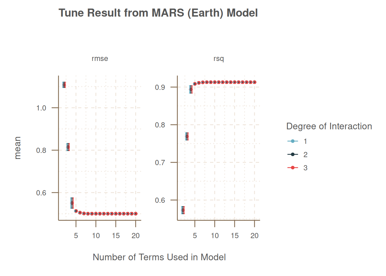
The original workflow which was initially set will be extracted. This is a very crucial step when comparing performance across different ML method.
mars_wf_extract <- extract_workflow(crop_tune)
mars_wf_extract
══ Workflow ════════════════════════════════════════════════════════════════════
Preprocessor: Recipe
Model: mars()
── Preprocessor ────────────────────────────────────────────────────────────────
3 Recipe Steps
• step_mutate()
• step_pca()
• step_dummy()
── Model ───────────────────────────────────────────────────────────────────────
MARS Model Specification (regression)
Main Arguments:
num_terms = tune()
prod_degree = tune()
Computational engine: earth To get the absolute model performance, rmse will be used instead of rsq when selecting the best tune parameter.
best_params <- select_best(crop_tune, metric = "rmse")Next, we combine both workflow and parameters together to get a finalized workflow.
crop_mars_wf <- finalize_workflow(
  mars_wf_extract,
  best_params
)

crop_mars_wf
══ Workflow ════════════════════════════════════════════════════════════════════
Preprocessor: Recipe
Model: mars()
── Preprocessor ────────────────────────────────────────────────────────────────
3 Recipe Steps
• step_mutate()
• step_pca()
• step_dummy()
── Model ───────────────────────────────────────────────────────────────────────
MARS Model Specification (regression)
Main Arguments:
num_terms = 8
prod_degree = 1
Computational engine: earth After getting our finalized we make the final model fit on the split object of our data.
crop_final_fit <- last_fit(
  crop_mars_wf,
  crop_yield_split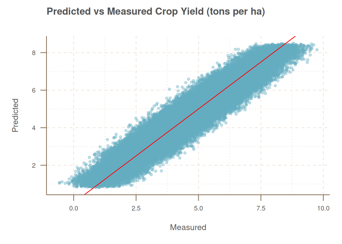
)We collect the metrics from our final model showing the predicted and observed data on the test of the split in Table 5. A goodness of fit test can be seen in Figure 5
crop_final_fit |>
  collect_metrics()
# A tibble: 2 × 4
.metric .estimator .estimate .config
<chr> <chr> <dbl> <chr>
1 rmse standard 0.500 pre0_mod0_post0
2 rsq standard 0.913 pre0_mod0_post0test_pred <- crop_final_fit |>
collect_predictions()
head(test_pred, n = 20) |>
knitr::kable()| .pred | id | yield_tons_per_hectare | .row | .config |
|---|---|---|---|---|
| 1.340249 | train/test split | 1.127443 | 3 | pre0_mod0_post0 |
| 5.939845 | train/test split | 5.898416 | 6 | pre0_mod0_post0 |
| 5.522160 | train/test split | 5.829542 | 8 | pre0_mod0_post0 |
| 2.943386 | train/test split | 2.943716 | 9 | pre0_mod0_post0 |
| 3.528423 | train/test split | 3.707293 | 10 | pre0_mod0_post0 |
| 6.046441 | train/test split | 6.525186 | 13 | pre0_mod0_post0 |
| 4.449305 | train/test split | 4.366881 | 17 | pre0_mod0_post0 |
| 5.248122 | train/test split | 4.858924 | 18 | pre0_mod0_post0 |
| 2.638067 | train/test split | 2.332255 | 26 | pre0_mod0_post0 |
| 5.130901 | train/test split | 4.876587 | 27 | pre0_mod0_post0 |
| 5.313136 | train/test split | 5.113588 | 31 | pre0_mod0_post0 |
| 4.919733 | train/test split | 4.898181 | 34 | pre0_mod0_post0 |
| 2.838416 | train/test split | 3.607496 | 36 | pre0_mod0_post0 |
| 4.897757 | train/test split | 4.696426 | 37 | pre0_mod0_post0 |
| 6.265479 | train/test split | 6.314786 | 40 | pre0_mod0_post0 |
| 2.830512 | train/test split | 2.368322 | 41 | pre0_mod0_post0 |
| 2.600831 | train/test split | 2.968063 | 44 | pre0_mod0_post0 |
| 6.220637 | train/test split | 6.654949 | 50 | pre0_mod0_post0 |
| 5.242452 | train/test split | 5.493174 | 53 | pre0_mod0_post0 |
| 6.313487 | train/test split | 6.411931 | 60 | pre0_mod0_post0 |
set.seed(3234)
#| label: fig-final-eval
#| fig-cap: Model evaluation measured vs predicted


test_pred |>
  janitor::clean_names() |>
  slice_sample(n = 100000) |>
  ggplot(aes(yield_tons_per_hectare, pred)) +
  geom_jitter(alpha = .4) +
  geom_abline(col = "red") +
  labs(
    x = "Measured",
    y = "Predicted",
    title = "Predicted vs Measured Crop Yield (tons per ha)"
  )
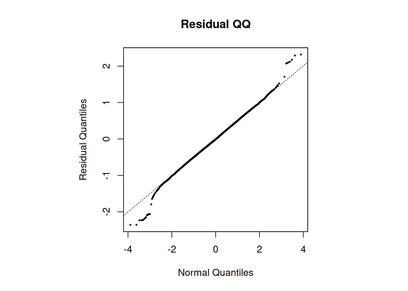
crop_final_fit |>
extract_fit_engine() |>
plot(3)
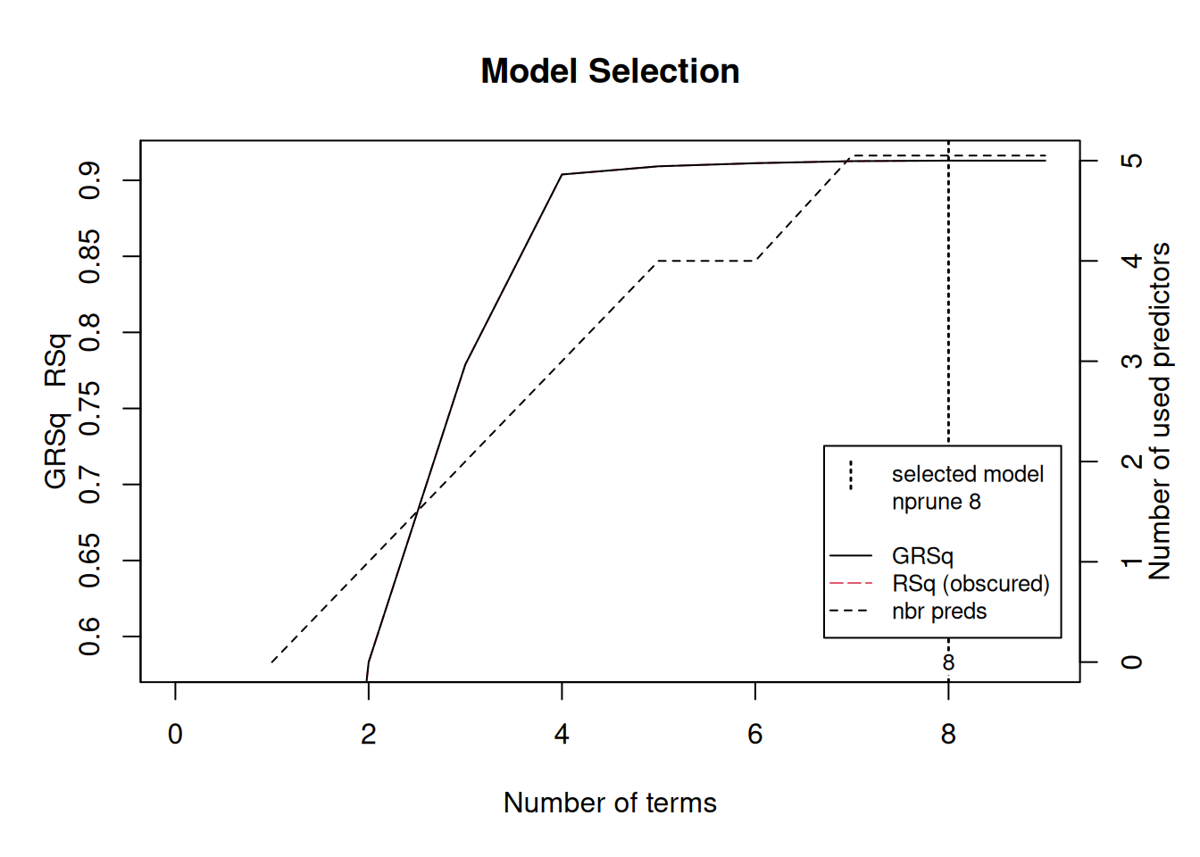
crop_final_fit |>
extract_fit_engine(4) |>
plot(1)
crop_final_fit |>
extract_fit_engine() |>
plot(4)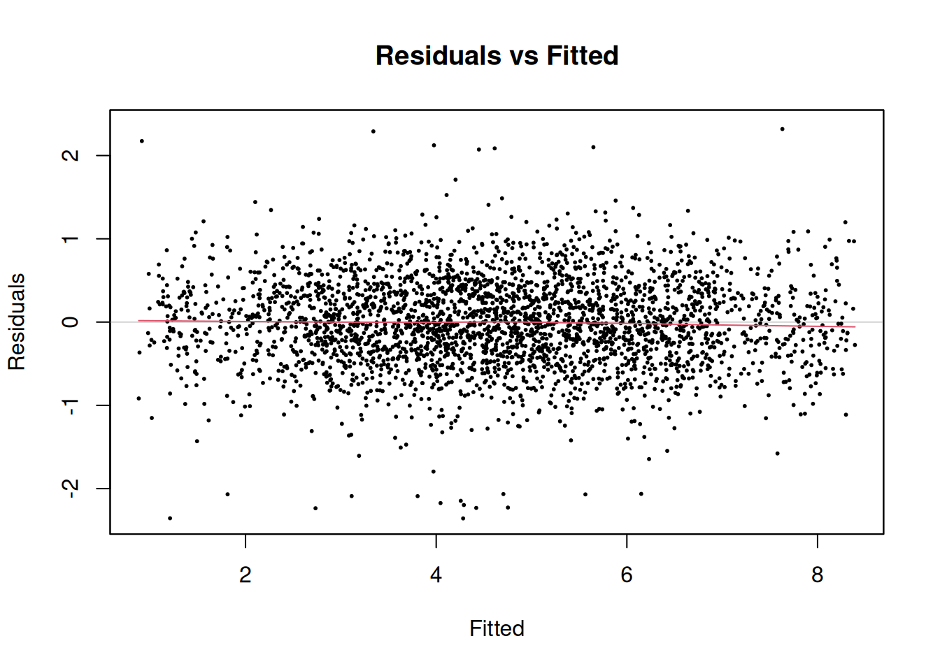
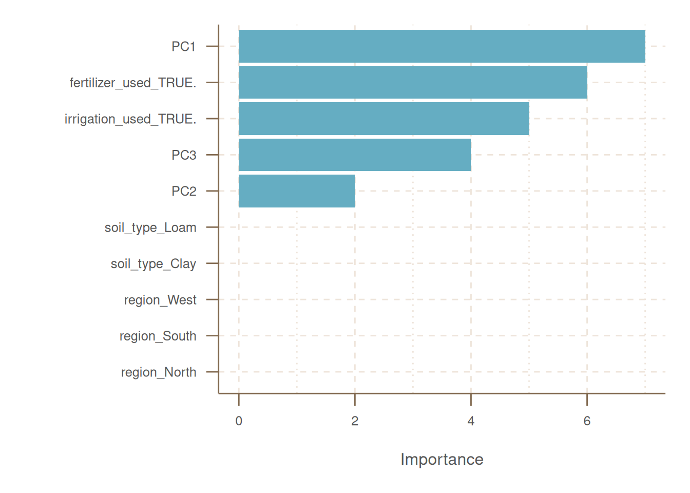
vip(
  crop_final_fit |>
    extract_fit_engine()
)