For this project, I will be using a K-Nearest Neighbors (KNN) machine learning algorithm to predict the types of forest in the forest type mapping data on UC Irvine ML repository. The data is a multi-temporal remote sensing data of a forested area collected using ASTER satellite imagery in Japan. Using this spectral data different forest types were mapped into for different classes:
Sugi forest (s)
Hinoki forest (h)
Mixed deciduous forest (d)
“Others”, that is non-forest land (o)
Load Packages and Data
To begin I will load the necessary packages and the dataset.
Warning: The `size` argument of `element_line()` is deprecated as of ggplot2 3.4.0.
ℹ Please use the `linewidth` argument instead.
ℹ The deprecated feature was likely used in the ggthemr package.
  Please report the issue to the authors.
Warning: The `size` argument of `element_rect()` is deprecated as of ggplot2 3.4.0.
ℹ Please use the `linewidth` argument instead.
ℹ The deprecated feature was likely used in the ggthemr package.
  Please report the issue to the authors.
Initial exploration and preview is necessary to understand the data.
Show the code
skimr::skim(forest_type_training)
Table 1: Data Summary
(a)
Name
forest_type_training
Number of rows
198
Number of columns
28
_______________________
Column type frequency:
character
1
numeric
27
________________________
Group variables
None
Variable type: character
(b)
skim_variable
n_missing
complete_rate
min
max
empty
n_unique
whitespace
class
0
1
1
1
0
4
0
Variable type: numeric
(c)
skim_variable
n_missing
complete_rate
mean
sd
p0
p25
p50
p75
p100
hist
b1
0
1
62.95
12.78
34.00
54.00
60.00
70.75
105.00
▂▇▃▂▁
b2
0
1
41.02
17.83
25.00
28.00
31.50
50.75
160.00
▇▂▁▁▁
b3
0
1
63.68
17.31
47.00
52.00
57.00
69.00
196.00
▇▂▁▁▁
b4
0
1
101.41
14.80
54.00
92.25
99.50
111.75
172.00
▁▇▆▁▁
b5
0
1
58.73
12.39
44.00
49.00
55.00
65.00
98.00
▇▅▂▁▁
b6
0
1
100.65
11.19
84.00
92.00
98.00
107.00
136.00
▇▇▅▂▁
b7
0
1
90.60
15.59
54.00
80.00
91.00
101.00
139.00
▂▆▇▃▁
b8
0
1
28.69
8.98
21.00
24.00
25.00
27.00
82.00
▇▁▁▁▁
b9
0
1
61.12
9.79
50.00
55.00
58.00
63.00
109.00
▇▂▁▁▁
pred_minus_obs_H_b1
0
1
50.82
12.84
7.66
40.67
53.03
59.92
83.32
▁▃▅▇▁
pred_minus_obs_H_b2
0
1
9.81
18.01
-112.60
0.27
18.80
22.26
29.79
▁▁▁▃▇
pred_minus_obs_H_b3
0
1
32.54
17.74
-106.12
27.20
37.61
43.33
55.97
▁▁▁▂▇
pred_minus_obs_H_b4
0
1
-3.90
15.08
-77.01
-15.92
-2.18
6.66
40.82
▁▁▆▇▁
pred_minus_obs_H_b5
0
1
-33.42
12.30
-73.29
-39.76
-29.16
-23.89
-19.49
▁▁▂▃▇
pred_minus_obs_H_b6
0
1
-40.45
10.87
-76.09
-46.16
-37.51
-32.94
-25.68
▁▁▃▆▇
pred_minus_obs_H_b7
0
1
-13.91
15.40
-62.74
-23.59
-14.84
-3.25
24.33
▁▂▇▅▂
pred_minus_obs_H_b8
0
1
1.01
9.07
-52.00
1.98
4.14
5.50
10.83
▁▁▁▁▇
pred_minus_obs_H_b9
0
1
-5.59
9.77
-53.53
-6.63
-2.26
0.25
5.74
▁▁▁▂▇
pred_minus_obs_S_b1
0
1
-20.04
4.95
-32.95
-23.33
-20.02
-17.79
5.13
▂▇▂▁▁
pred_minus_obs_S_b2
0
1
-1.01
1.78
-8.80
-1.86
-0.97
-0.04
12.46
▁▇▃▁▁
pred_minus_obs_S_b3
0
1
-4.36
2.35
-11.21
-5.79
-4.35
-2.88
7.37
▁▇▆▁▁
pred_minus_obs_S_b4
0
1
-21.00
6.49
-40.37
-24.09
-20.46
-17.95
1.88
▁▃▇▁▁
pred_minus_obs_S_b5
0
1
-0.97
0.70
-3.27
-1.29
-0.94
-0.64
3.44
▁▇▂▁▁
pred_minus_obs_S_b6
0
1
-4.60
1.74
-8.73
-5.75
-4.54
-3.62
3.94
▂▇▃▁▁
pred_minus_obs_S_b7
0
1
-18.84
5.25
-34.14
-22.24
-19.20
-16.23
3.67
▁▇▆▁▁
pred_minus_obs_S_b8
0
1
-1.57
1.81
-8.87
-2.37
-1.42
-0.66
8.84
▁▅▇▁▁
pred_minus_obs_S_b9
0
1
-4.16
1.98
-10.83
-5.12
-4.12
-3.11
7.79
▁▇▃▁▁
Result from Table 1 (a) shows that the data is having one character variable, our target variable class and the rest are numeric. There are no missing data in the data for the target variable, Table 1 (b), and the features, Table 1 (c).
Exploratory Data Analysis
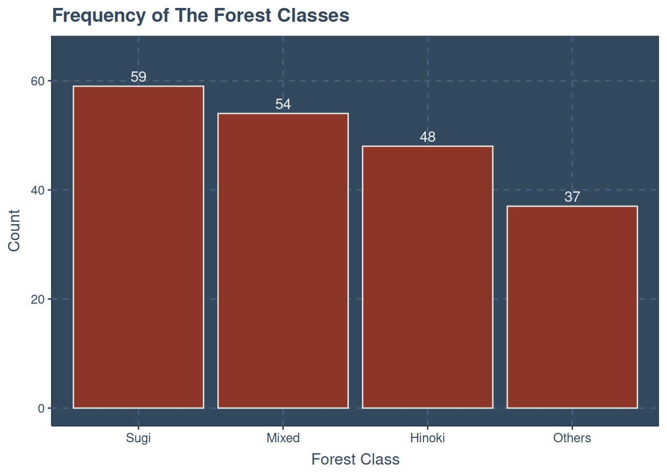
A quick check on the number of occurrence for each forest class is given below
Show the code
forest_type_training |>mutate(class =case_when( class =="d"~"Mixed", class =="s"~"Sugi", class =="h"~"Hinoki",.default ="Others" ) ) |>ggplot(aes(fct_infreq(class))) +geom_bar(col ="gray90",fill ="tomato4" ) +geom_text(aes(y =after_stat(count),label =after_stat(count)),stat ="count",vjust =-.4 ) +labs(x ="Forest Class",y ="Count",title ="Frequency of The Forest Classes" ) +expand_limits(y =c(0, 65)) +guides(fill ="none")
Figure 1: Frequency of Forest Classee
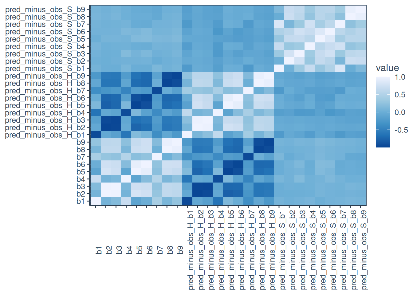
Furthermore, Figure 2 hows the heatmap of the numeric variables
K-Nearest Neighbor Model Specification (classification)

Main Arguments:
  neighbors = tune()
  dist_power = tune()

Computational engine: kknn

Model fit template:
kknn::train.kknn(formula = missing_arg(), data = missing_arg(),
    ks = min_rows(tune(), data, 5), distance = tune())
Feature Engineering
K-NN requires quite the preprocessing due to Euclidean distance being sensitive to outliers, as distance measures are sensitive to the scale of the features. To prevent bias from the different features and allowing large predictors contribute the most to the distance between samples I will use the following preprocessing step:
To ensure we get the best value for k, that is the neighbors and the right type of distance metric to use, Minkowski distance to determine if Manhattan or Euclidean will be optimal.
Warning: The `scale_name` argument of `discrete_scale()` is deprecated as of ggplot2
3.5.0.
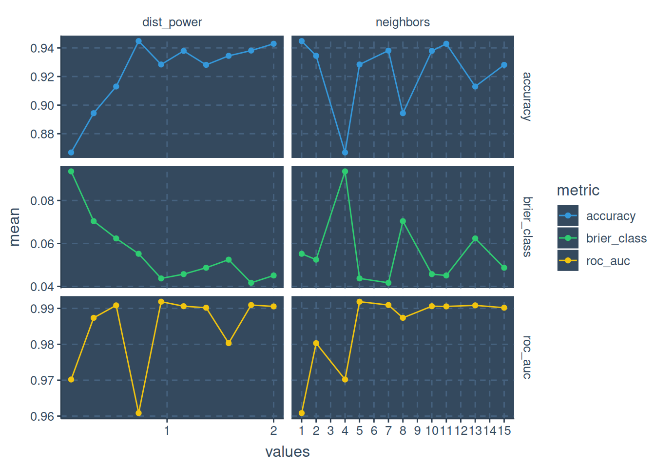
Figure 3: Tune Result
The three evaluation metrics have high mean at different points, roc_auc and accuracy has their best mean at neighbor = 11 and distance power = 2 while brier class or score is having it’s best neighbor at 5 and distance power at 0.9444444.
Since I am interested in how well the model distinguishes between the ranking of the classes, I will use the roc_auc. Given that, we will fit the best parameter based on roc_auc to the workflow.
          Truth
Prediction   d   h   o   s
         d  89   0   9  13
         h   1  33   0  11
         o   3   0  34   0
         s  12   5   3 112
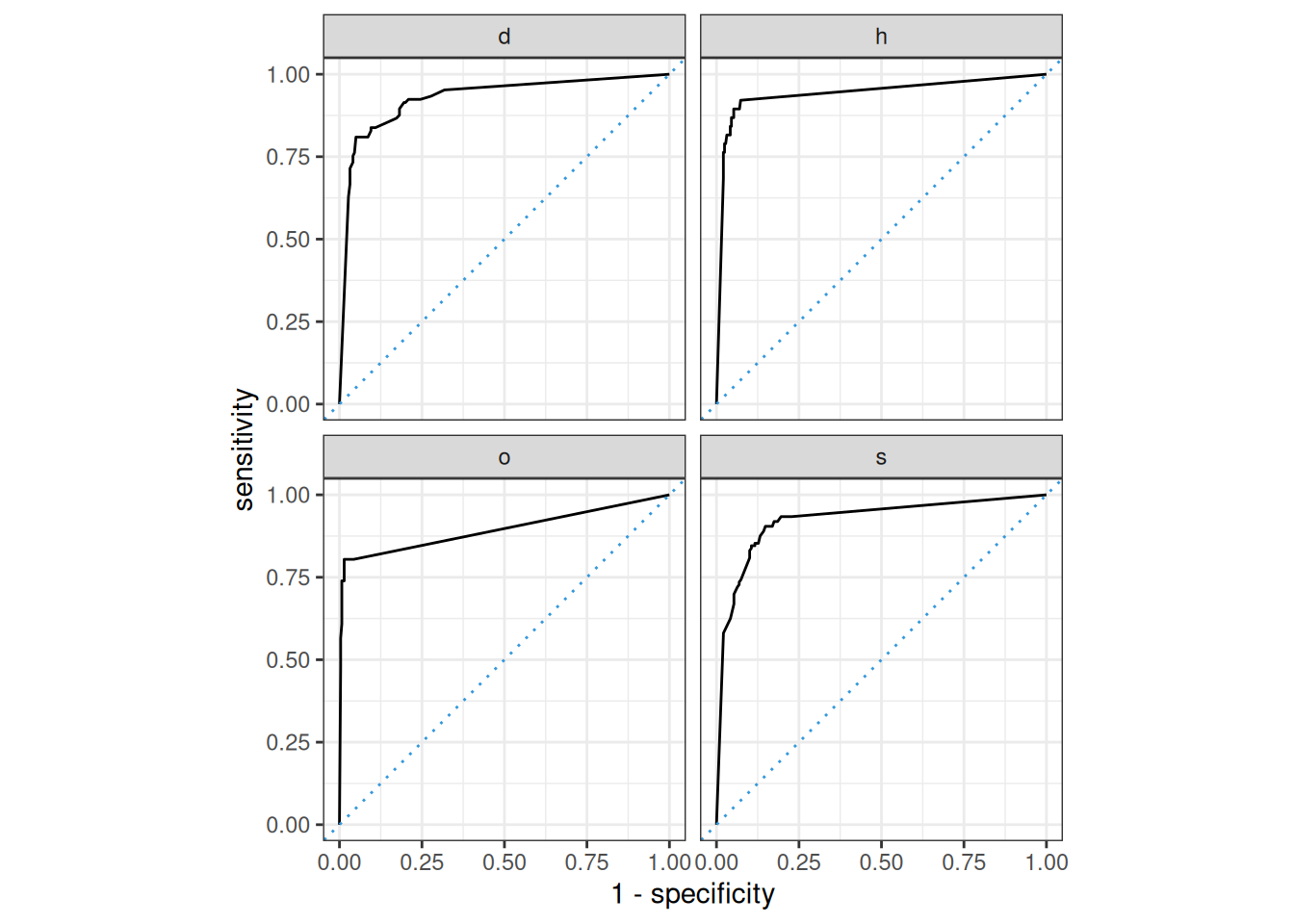
## Conclusion After fitting the final K-NN workflow on the training data and predicting on the test set, we calculated the ROC AUC to evaluate the model’s classification performance based on the predicted probabilities. The ROC AUC helps assess how well the model discriminates between the different classes. For multi-class classification, the AUC can be computed for each class to assess overall performance.
The plotted ROC curve visually represents the trade-off between the true positive rate (sensitivity) and the false positive rate at different threshold settings, giving further insight into how well the model separates the classes.
An AUC of 0.93 indicates a very good discriminatory power. Based on the ROC curve and AUC score, the model is well suited for classification tasks.