pacman::p_load(
  tidymodels, tidyverse, ggthemr, farff, gt,
  earth, rpart.plot, vip, corrplot, skimr
)

ggthemr(
  palette = "flat dark",
  layout = "clean",
  spacing = 2,
  type = "outer"
)

darken_swatch(amount = .1)
additional_colors <- c("#af4242", "#535364", "#FFC300", "#e09263", "#123367", "salmon", "#c0ca33", "#689f38", "#e53935")

set_swatch(c(unique(swatch()), additional_colors))Introduction
The aim of this blog post is to use decision tree machine learning algorithm to classify dry bean based on some features. This is a Kaggle challenge dataset. Images of 13,611 grains of 7 different registered dry beans were taken with a high-resolution camera. A total of 16 features; 12 dimensions and 4 shape forms, were obtained from the grains. The features of the data are:
| Feature | Description |
|---|---|
| Area (A) | The area of a bean zone and the number of pixels within its boundaries. |
| Perimeter (P) | Bean circumference is defined as the length of its border. |
| Major axis length (L) | The distance between the ends of the longest line that can be drawn from a bean. |
| Minor axis length (l) | The longest line that can be drawn from the bean while standing perpendicular to the main axis. |
| Aspect ratio (K) | Defines the relationship between L and l. |
| Eccentricity (Ec) | Eccentricity of the ellipse having the same moments as the region. |
| Convex area (C) | Number of pixels in the smallest convex polygon that can contain the area of a bean seed. |
| Equivalent diameter (Ed) | The diameter of a circle having the same area as a bean seed area. |
| Extent (Ex) | The ratio of the pixels in the bounding box to the bean area. |
| Solidity (S) | Also known as convexity. The ratio of the pixels in the convex shell to those found in beans. |
| Roundness (R) | Calculated with the following formula: (4piA)/(P^2) |
| Compactness (CO) | Measures the roundness of an object: Ed/L |
| ShapeFactor1 (SF1) | |
| ShapeFactor2 (SF2) | |
| ShapeFactor3 (SF3) | |
| ShapeFactor4 (SF4) | |
| Class | Seker, Barbunya, Bombay, Cali, Dermosan, Horoz and Sira |
Load Packages
To begin, we load the necessary packages. I also set the extra swatch color, just in case we have more than the default provided by ggthemr. I have recently fell in love with using the ggthemr package by Mikata-Project.
This is the first time I am seeing a data with a .arffextension, so, I searched online immediately to see if there’s a package to import a data with an arff extension in R. The best place to search for this is CRAN, of course Google will also give very good result, but I choose CRAN regardless. Fortunately, there’s the farrf package with development starting in 2015 by mlr-org. The package is also pretty straightforward to use. Interestingly the package imports data as data.frame, which is great. Afterwards, I converted to tibble.
bean_tbl <- readARFF("data/Dry_Bean_Dataset.arff") |>
  janitor::clean_names() |>
  as_tibble()

head(bean_tbl)
# A tibble: 6 × 17
area perimeter major_axis_length minor_axis_length aspect_ration eccentricity
<dbl> <dbl> <dbl> <dbl> <dbl> <dbl>
1 28395 610. 208. 174. 1.20 0.550
2 28734 638. 201. 183. 1.10 0.412
3 29380 624. 213. 176. 1.21 0.563
4 30008 646. 211. 183. 1.15 0.499
5 30140 620. 202. 190. 1.06 0.334
6 30279 635. 213. 182. 1.17 0.520
# ℹ 11 more variables: convex_area <dbl>, equiv_diameter <dbl>, extent <dbl>,
# solidity <dbl>, roundness <dbl>, compactness <dbl>, shape_factor1 <dbl>,
# shape_factor2 <dbl>, shape_factor3 <dbl>, shape_factor4 <dbl>, class <fct>Exploratory Datta Analysis
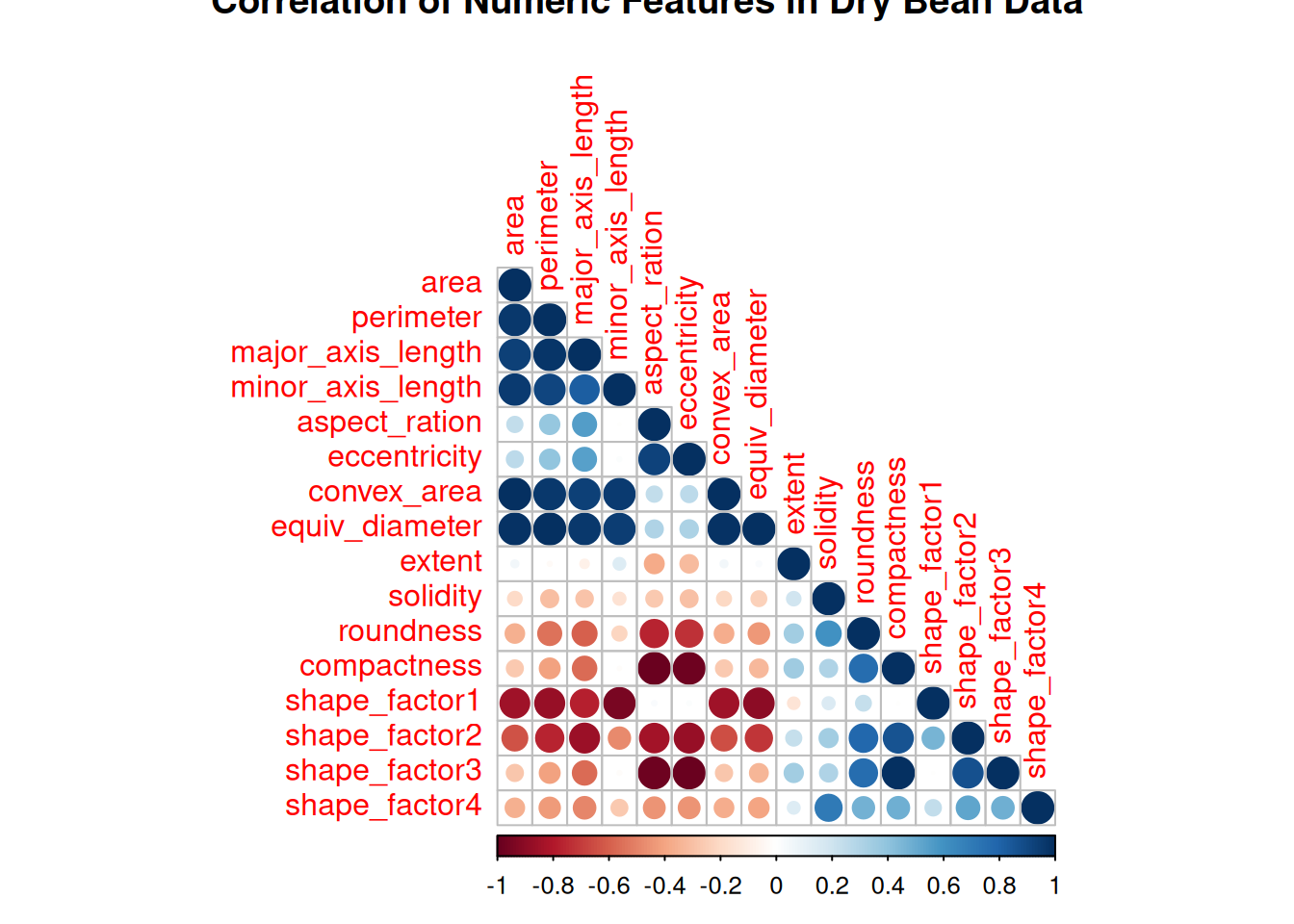
Next is EDA, this will be quick and short. Table 1 shows a good summary of the data including the data types, and information on the completeness of the data. From what the result in Table 1 (a) and Table 1 (b) the data is complete. Figure 1 shows the correlation matrix of the numeric variables.
skim(bean_tbl)| Name | bean_tbl |
| Number of rows | 13611 |
| Number of columns | 17 |
| _______________________ | |
| Column type frequency: | |
| factor | 1 |
| numeric | 16 |
| ________________________ | |
| Group variables | None |
Variable type: factor
| skim_variable | n_missing | complete_rate | ordered | n_unique | top_counts |
|---|---|---|---|---|---|
| class | 0 | 1 | FALSE | 7 | DER: 3546, SIR: 2636, SEK: 2027, HOR: 1928 |
Variable type: numeric
| skim_variable | n_missing | complete_rate | mean | sd | p0 | p25 | p50 | p75 | p100 | hist |
|---|---|---|---|---|---|---|---|---|---|---|
| area | 0 | 1 | 53048.28 | 29324.10 | 20420.00 | 36328.00 | 44652.00 | 61332.00 | 254616.00 | ▇▂▁▁▁ |
| perimeter | 0 | 1 | 855.28 | 214.29 | 524.74 | 703.52 | 794.94 | 977.21 | 1985.37 | ▇▆▁▁▁ |
| major_axis_length | 0 | 1 | 320.14 | 85.69 | 183.60 | 253.30 | 296.88 | 376.50 | 738.86 | ▇▆▂▁▁ |
| minor_axis_length | 0 | 1 | 202.27 | 44.97 | 122.51 | 175.85 | 192.43 | 217.03 | 460.20 | ▇▇▁▁▁ |
| aspect_ration | 0 | 1 | 1.58 | 0.25 | 1.02 | 1.43 | 1.55 | 1.71 | 2.43 | ▂▇▅▂▁ |
| eccentricity | 0 | 1 | 0.75 | 0.09 | 0.22 | 0.72 | 0.76 | 0.81 | 0.91 | ▁▁▂▇▇ |
| convex_area | 0 | 1 | 53768.20 | 29774.92 | 20684.00 | 36714.50 | 45178.00 | 62294.00 | 263261.00 | ▇▂▁▁▁ |
| equiv_diameter | 0 | 1 | 253.06 | 59.18 | 161.24 | 215.07 | 238.44 | 279.45 | 569.37 | ▇▆▁▁▁ |
| extent | 0 | 1 | 0.75 | 0.05 | 0.56 | 0.72 | 0.76 | 0.79 | 0.87 | ▁▁▅▇▂ |
| solidity | 0 | 1 | 0.99 | 0.00 | 0.92 | 0.99 | 0.99 | 0.99 | 0.99 | ▁▁▁▁▇ |
| roundness | 0 | 1 | 0.87 | 0.06 | 0.49 | 0.83 | 0.88 | 0.92 | 0.99 | ▁▁▂▇▇ |
| compactness | 0 | 1 | 0.80 | 0.06 | 0.64 | 0.76 | 0.80 | 0.83 | 0.99 | ▂▅▇▂▁ |
| shape_factor1 | 0 | 1 | 0.01 | 0.00 | 0.00 | 0.01 | 0.01 | 0.01 | 0.01 | ▁▃▇▃▁ |
| shape_factor2 | 0 | 1 | 0.00 | 0.00 | 0.00 | 0.00 | 0.00 | 0.00 | 0.00 | ▇▇▇▃▁ |
| shape_factor3 | 0 | 1 | 0.64 | 0.10 | 0.41 | 0.58 | 0.64 | 0.70 | 0.97 | ▂▇▇▃▁ |
| shape_factor4 | 0 | 1 | 1.00 | 0.00 | 0.95 | 0.99 | 1.00 | 1.00 | 1.00 | ▁▁▁▁▇ |
corrplot(
  cor(bean_tbl[, 1:16]),
  method = "circle",
  addrect = 2,
  pch = 5,
  title = "Correlation of Numeric Features in Dry Bean Data",
  type = "lower"
)
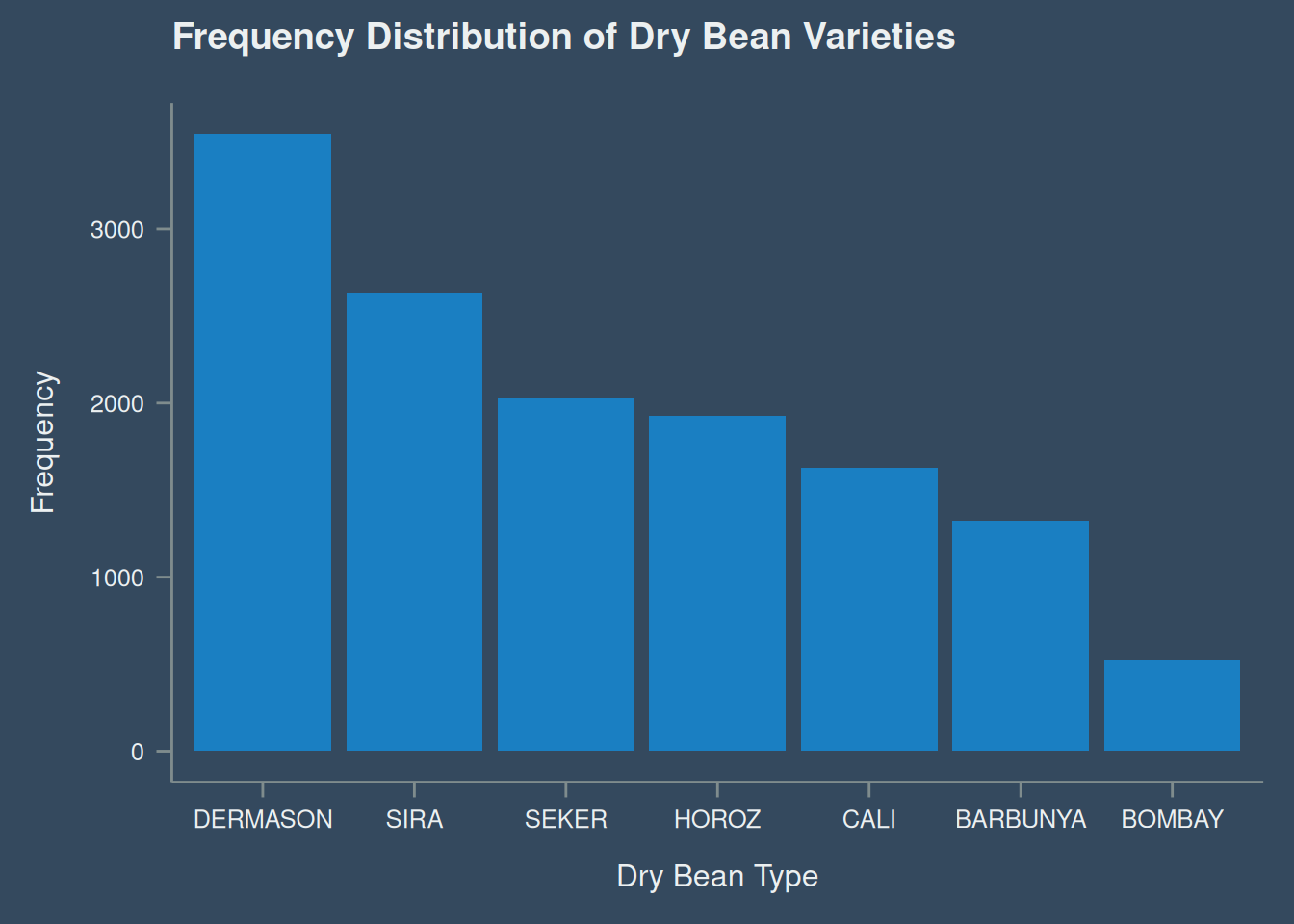
The frequency of the different types of dry bean is shown in Figure 2.
bean_tbl |>
  ggplot(aes(fct_infreq(class))) +
  geom_bar() +
  labs(
    x = "Dry Bean Type",
    y = "Frequency",
    title = "Frequency Distribution of Dry Bean Varieties"
  )
Modeling
Data Shairing
The data was split to two, a testing data, which is 30% the number of records of the original data and 70% for the training data. To ensure reproducibility, a seed was set.
set.seed(122)
bean_split <- initial_split(bean_tbl, prop = .7, strata = class)
bean_split
<Training/Testing/Total>
<9525/4086/13611>bean_train <- training(bean_split)Resamples of the training data was also set at 10 folds, which I think has continuously been the go-to value for number of folds.
bean_folds <- vfold_cv(bean_train, v = 10)Model Specification
As stated earlier, decision tree model will be used in this post.
dt_spec <- decision_tree(
  cost_complexity = tune(),
  tree_depth = tune(),
  min_n = tune()
) |>
  set_mode("classification") |>
  set_engine("rpart")

dt_spec
Decision Tree Model Specification (classification)
Main Arguments:
cost_complexity = tune()
tree_depth = tune()
min_n = tune()
Computational engine: rpart Decision trees does not require a lot of preprocessing. So, the stating the family will be the only preprocessing step.
dt_rec <- recipe(class ~ ., data = bean_train)
dt_wf <- workflow() |>
add_recipe(dt_rec) |>
add_model(dt_spec)
dt_wf══ Workflow ════════════════════════════════════════════════════════════════════
Preprocessor: Recipe
Model: decision_tree()
── Preprocessor ────────────────────────────────────────────────────────────────
0 Recipe Steps
── Model ───────────────────────────────────────────────────────────────────────
Decision Tree Model Specification (classification)

Main Arguments:
  cost_complexity = tune()
  tree_depth = tune()
  min_n = tune()

Computational engine: rpart Model Tuning
After model specification, a grid can be randomly generated from the tune parameters.
set.seed(122)

dt_grid <- dt_spec |>
  extract_parameter_set_dials() |>
  grid_random(size = 20)

dt_grid |> gt() |>
  tab_header(md("**Parameter Grid for Tuning**")) |>
  cols_label(
    cost_complexity = md("**Cost Complexity**"),
    tree_depth = md("**Tree Depth**"),
    min_n = md("**Min Node**")
  ) |>
  cols_align(align = "left") |>
opt_stylize(style = 4, color = "gray")| Parameter Grid for Tuning | ||
|---|---|---|
| Cost Complexity | Tree Depth | Min Node |
| 1.396964e-02 | 12 | 29 |
| 1.450966e-02 | 6 | 39 |
| 5.187936e-09 | 3 | 16 |
| 2.334592e-10 | 6 | 27 |
| 1.628025e-05 | 10 | 38 |
| 4.280073e-05 | 6 | 5 |
| 1.301318e-04 | 4 | 12 |
| 1.059508e-10 | 7 | 35 |
| 2.098525e-10 | 2 | 4 |
| 2.343786e-05 | 4 | 10 |
| 2.170993e-02 | 7 | 20 |
| 1.934008e-07 | 4 | 8 |
| 3.608012e-05 | 12 | 4 |
| 9.567531e-05 | 5 | 9 |
| 5.905851e-05 | 6 | 30 |
| 1.786420e-10 | 9 | 8 |
| 2.587232e-09 | 10 | 21 |
| 1.647915e-05 | 15 | 2 |
| 3.866406e-07 | 3 | 27 |
| 4.274980e-09 | 9 | 3 |
After the ground works are down. The parameter needs to be tuned.
dt_tune <- tune_grid(
  object = dt_wf,
  resamples = bean_folds,
  grid = dt_grid,
  control = control_grid(save_pred = TRUE, save_workflow = TRUE)
)
Results from tuning is shown in Table 2 with, represented visually in Figure 4 three metrics to measure which combination of the parameters would give the best result.
dt_tune |>
  collect_metrics()
# A tibble: 60 × 9
cost_complexity tree_depth min_n .metric .estimator mean n std_err
<dbl> <int> <int> <chr> <chr> <dbl> <int> <dbl>
1 1.06e-10 7 35 accuracy multiclass 0.893 10 0.00270
2 1.06e-10 7 35 brier_class multiclass 0.0808 10 0.00215
3 1.06e-10 7 35 roc_auc hand_till 0.984 10 0.000989
4 1.79e-10 9 8 accuracy multiclass 0.903 10 0.00298
5 1.79e-10 9 8 brier_class multiclass 0.0769 10 0.00260
6 1.79e-10 9 8 roc_auc hand_till 0.981 10 0.00147
7 2.10e-10 2 4 accuracy multiclass 0.649 10 0.00230
8 2.10e-10 2 4 brier_class multiclass 0.225 10 0.00103
9 2.10e-10 2 4 roc_auc hand_till 0.820 10 0.00112
10 2.33e-10 6 27 accuracy multiclass 0.891 10 0.00253
# ℹ 50 more rows
# ℹ 1 more variable: .config <chr>Visually, this is represented below:
dt_tune |>
  collect_metrics() |>
  pivot_longer(
    cols = cost_complexity:min_n,
    names_to = "params",
    values_to = "values"
  ) |>
  ggplot(aes(values, mean, colour = .metric)) +
  geom_point() +
  geom_line() +
  facet_grid(.metric~params, scales = "free")
Warning: The `scale_name` argument of `discrete_scale()` is deprecated as of ggplot2
3.5.0.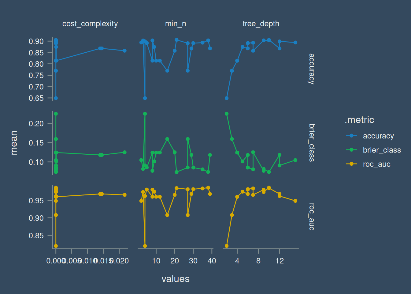
Final FIt
Next we extract the best combination of the parameters using roc_auc as the evaluation metric.
best_tune <- dt_tune |>
  select_best(metric = "roc_auc")

best_tune
# A tibble: 1 × 4
cost_complexity tree_depth min_n .config
<dbl> <int> <int> <chr>
1 0.0000163 10 38 pre0_mod10_post0Next, we refit the best tune parameter to the workflow.
dt_wf <- dt_tune |>
  extract_workflow()

dt_fwf <- finalize_workflow(
  dt_wf,
  best_tune
)

dt_fwf
══ Workflow ════════════════════════════════════════════════════════════════════
Preprocessor: Recipe
Model: decision_tree()
── Preprocessor ────────────────────────────────────────────────────────────────
0 Recipe Steps
── Model ───────────────────────────────────────────────────────────────────────
Decision Tree Model Specification (classification)
Main Arguments:
cost_complexity = 1.62802544691579e-05
tree_depth = 10
min_n = 38
Computational engine: rpart dt_final_fit <- dt_fwf |>
last_fit(bean_split)A visualization of how the features are used in determining the class of the dry-beans is shown in Figure 5.
dt_final_fit |>
  extract_fit_engine() |>
  rpart.plot::rpart.plot()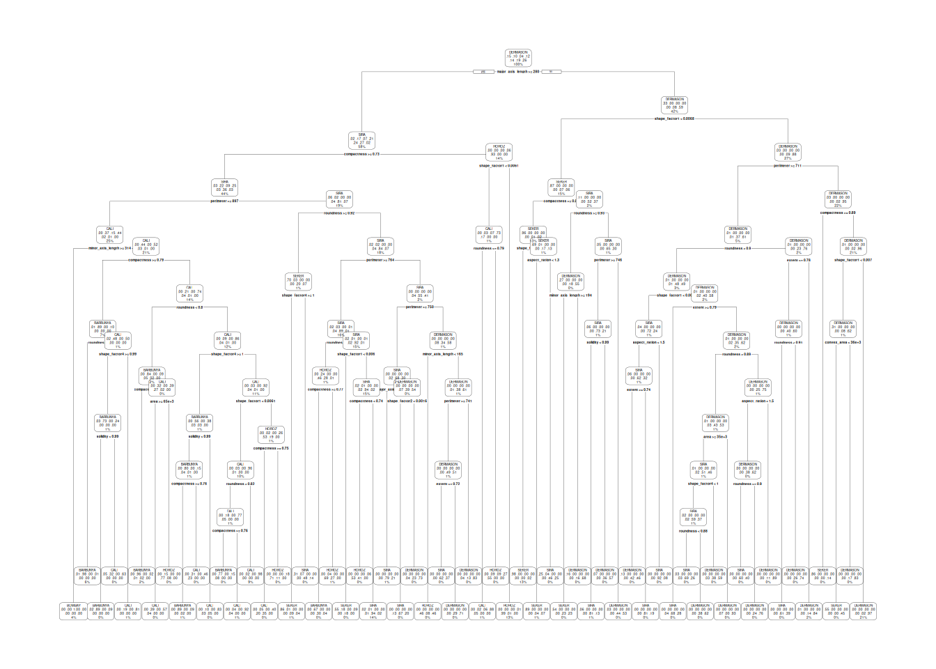
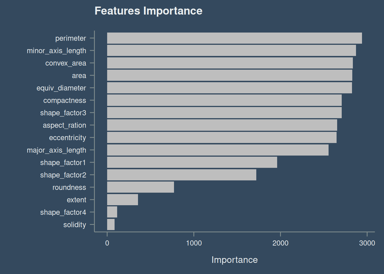
Variable Importance Plot
The feature perimeter have the largest effect on the model, while solidity have the least effect. Check Figure 6
dt_final_fit |>
  extract_fit_engine() |>
  vip(
    geom = "col",
    num_features = 17,
    aesthetics = list(
      fill = "gray",
      size = 1.5
    )
  ) +
  ggtitle("Features Importance")
Warning in (function (mapping = NULL, data = NULL, stat = "identity", position
= "stack", : Ignoring unknown parameters: `size`