Heavy or Light: Can Visualization help to Identify Thinning Frequency and Intensity?

This post aims to visualize the development of two species: Birch (Betula pubescens) and Norway spruce (Picea abies). The visualization would give insight into what type of thinning operation has been carried out.

Pine Plantation. Photo by Simon Rizzi - Pexels.com

I will answer the following questions using graphs:

• What is the total volume for each species
• How many thinnings were made
• What is the total yield (easy to mistake, but it’s different from total volume)
• Were thinnings made heavy or light

library(tidyverse)
library(ggthemr)
ggthemr(
  palette = "earth",
  layout = "scientific",
  spacing = 2,
  type = "outer"
)

Warning: The `size` argument of `element_line()` is deprecated as of ggplot2 3.4.0.
ℹ Please use the `linewidth` argument instead.
ℹ The deprecated feature was likely used in the ggthemr package.
  Please report the issue to the authors.

Warning: The `size` argument of `element_rect()` is deprecated as of ggplot2 3.4.0.
ℹ Please use the `linewidth` argument instead.
ℹ The deprecated feature was likely used in the ggthemr package.
  Please report the issue to the authors.

The Data

Data Description

• age: the age of the stand

• site: the site number (1 for spruce and 6 birch)

• stdens: stem density (st/ha)

• ba: basal area (m²/ha)

• spruce_dgv: quadratic mean dbh for spruce in cm

• birch_dgv: quadratic mean dbh for birch in cm

• stand_vol: standing volume

• harv_vol: harvested volume

• mor_vol: mortality volume in m³ at the age

The data for this post is available here.

std_tbl <- read_table("https://raw.githubusercontent.com/xrander/SLU-Plantation-Experimentation/master/Data/Lab%204/lab4mai%20(2).txt") |> 
  janitor::clean_names()

After importing the data, a good first step is to understand the structure of the data.

str(std_tbl)

spc_tbl_ [50 × 9] (S3: spec_tbl_df/tbl_df/tbl/data.frame)
 $ site      : num [1:50] 1 1 1 1 1 1 1 1 1 1 ...
 $ age       : num [1:50] 5 10 15 20 25 30 35 40 45 50 ...
 $ stdens    : num [1:50] 2019 1999 1985 1970 1948 ...
 $ ba        : num [1:50] 0.0834 1.7468 7.0915 14.9834 22.4206 ...
 $ stand_vol : num [1:50] 0.6 4.5 22.5 66.8 126.6 ...
 $ harv_vol  : num [1:50] 0 0 0 0 0 ...
 $ mor_vol   : num [1:50] 0 0.01 0.03 0.15 0.64 1.44 2.74 4.25 3.77 3.31 ...
 $ spruce_dgv: num [1:50] 1.35 3.8 7.18 10.32 12.73 ...
 $ birch_dgv : num [1:50] 0 0 0 0 0 0 0 0 0 0 ...
 - attr(*, "spec")=
  .. cols(
  ..   `"site"` = col_double(),
  ..   `"age"` = col_double(),
  ..   `"stdens"` = col_double(),
  ..   `"ba"` = col_double(),
  ..   `"stand_vol"` = col_double(),
  ..   `"harv_vol"` = col_double(),
  ..   `"mor_vol"` = col_double(),
  ..   `"spruce_dgv"` = col_double(),
  ..   `"birch_dgv"` = col_double()
  .. )

To get a high-level summary of the data, I will use skimr (This should help better under stand the data).

skimr::skim_without_charts(std_tbl)

Table 1: Data Summary

Data summary

Name	std_tbl
Number of rows	50
Number of columns	9
_______________________
Column type frequency:
numeric	9
________________________
Group variables	None

Variable type: numeric

skim_variable	n_missing	complete_rate	mean	sd	p0	p25	p50	p75	p100
site	0	1	3.50	2.53	1.00	1.00	3.50	6.00	6.00
age	0	1	65.00	36.42	5.00	35.00	65.00	95.00	125.00
stdens	0	1	1124.47	594.83	340.90	540.08	943.40	1675.30	2018.60
ba	0	1	30.31	12.47	0.08	25.31	32.86	38.58	49.11
stand_vol	0	1	336.60	181.81	0.60	206.70	367.90	462.15	648.40
harv_vol	0	1	13.65	47.93	0.00	0.00	0.00	0.00	225.92
mor_vol	0	1	6.35	5.94	0.00	2.83	4.48	8.12	24.32
spruce_dgv	0	1	18.90	18.41	0.00	4.99	11.59	33.67	55.85
birch_dgv	0	1	12.17	9.21	0.00	6.45	9.71	19.86	28.33

From Table 1, we can see that there are no missing data (n-missing = 0 and complete_rate = 1).

There are some variables that are not numerical but are categorical variables coded as numbers. Section 1.1 shows that site 1 represents Spruce and site 6 Birch. I will create a new variable that holds a factor of the species.

std_tbl <- std_tbl |> 
  mutate(
    species = case_when(
      site == 6 ~ "Birch",
      site == 1 ~ "Spruce"
    ),
    species = factor(species),
    .after = age
  )

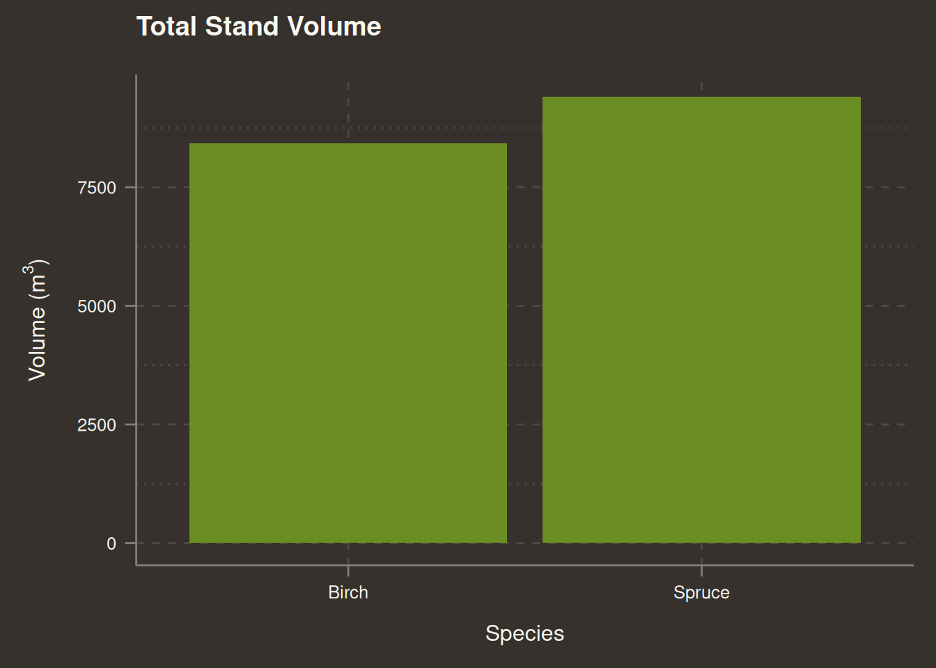
Total Volume Estimation

To estimate the total volume, we need to sum up all volume data in the data stand_vol, harv_vol, and mor_vol

\[totvol = standvol + harvol + morvol\]

std_tbl <-std_tbl |> 
  mutate(
    tot_vol = stand_vol + harv_vol + mor_vol,
    .after = ba
  )

Figure 1 shows that Spruce has a higher volume than Birch.

std_tbl |> 
  ggplot(aes(species, tot_vol)) +
  geom_col(fill = "olivedrab") +
  labs(
    x = "Species",
    y = expression(paste("Volume (", m^{3}, ")", sep = "")),
    title = "Total Stand Volume"
  )

Figure 1: Total volume(\(m^3\)) of stand

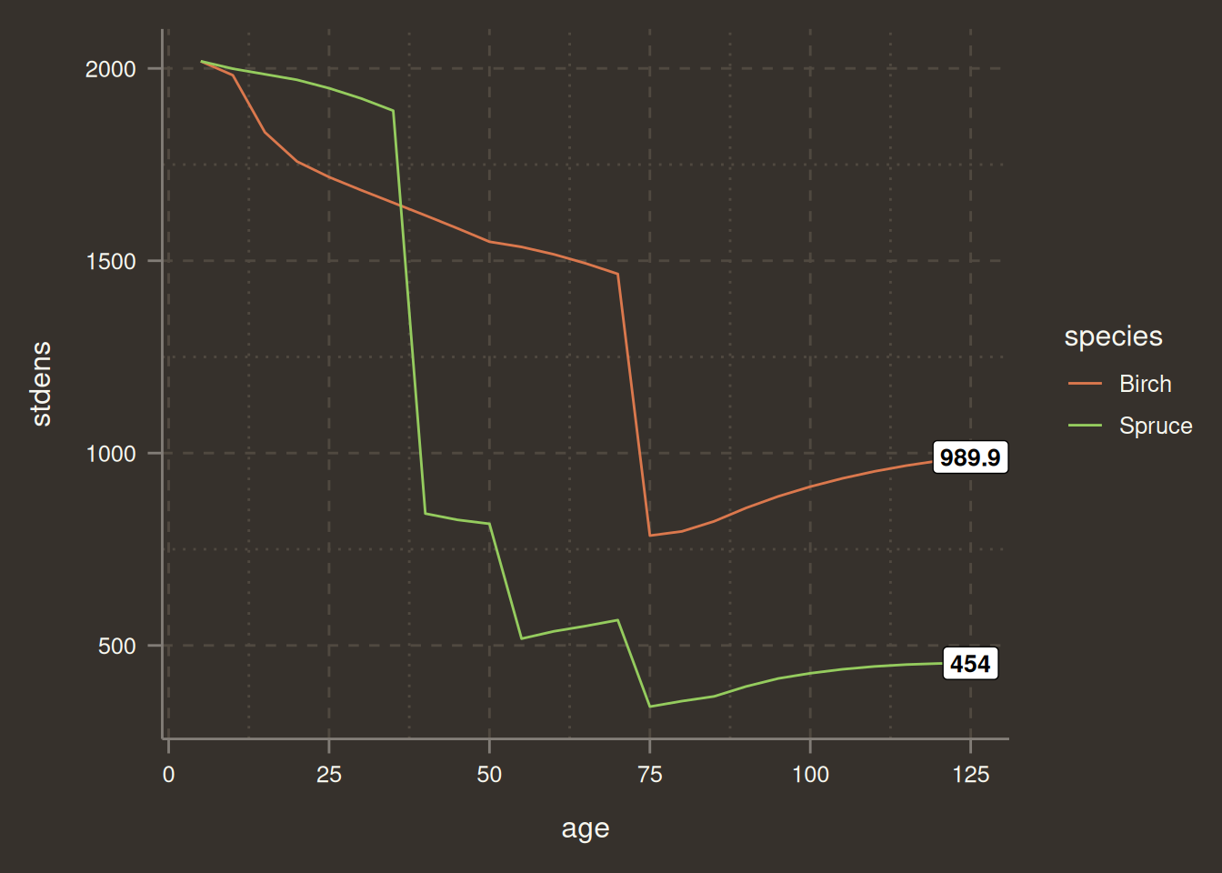
If we look at Figure 2, we see that both species had a planting density of 2000 st/ha and had several interventions with density at 125 years old at 989.9 st/ha for Birch and 454 st/ha for Spruce. This confirms that harvesting/thinning has been done at certain points or mortality has occurred in the stand

max_age_ext <- std_tbl |> filter(age == max(age))

std_tbl |> 
  ggplot(aes(age, stdens, col = species)) +
  # geom_point(size = .3) +
  geom_line() +
  geom_label(
    data = max_age_ext,
    aes(age, stdens, label = stdens),
    color = "black",
    size = 3.5,fontface = "bold",
    show.legend = FALSE
  )

Warning: The `scale_name` argument of `discrete_scale()` is deprecated as of ggplot2
3.5.0.

Figure 2: Stand density trend over time

Thinning Investigation

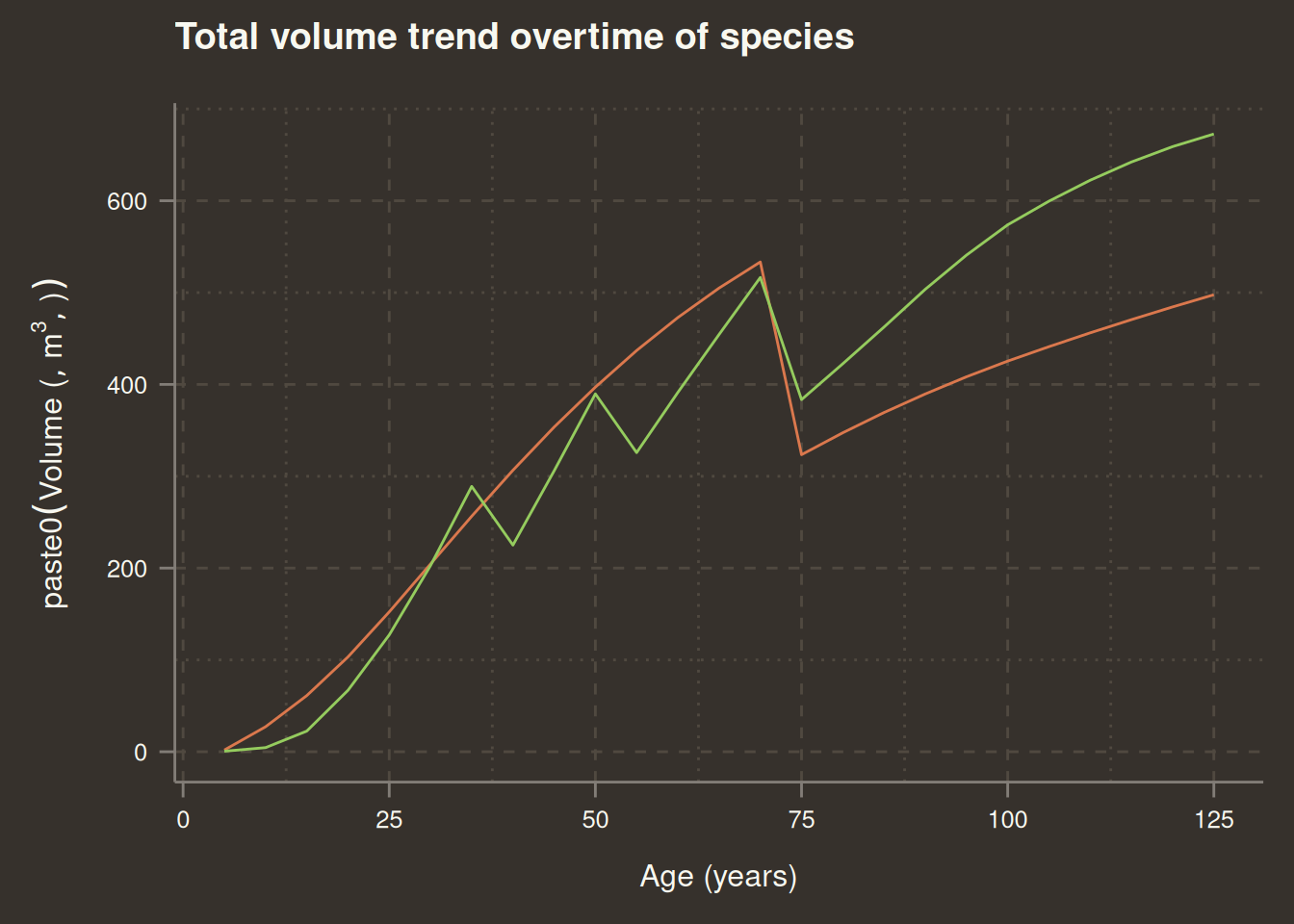
Plotting total volume against age should show the trend of stand development; any significant dip in development is where a thinning operation has occurred. Figure 3 shows that there’s been a single thinning in the Birch stand, while we have three thinnings in the Spruce stand. Are the thinnings heavy or not? We can’t say at the moment. Let’s move on to estimate the yield for both stands, then we will answer this question later.

std_tbl |> 
  ggplot(aes(age, tot_vol, colour = species)) + 
  geom_line(show.legend=FALSE) +
  labs(
    x = "Age (years)",
    y = expression(paste0("Volume (", m^{3}, ")")),
    title = "Total volume trend overtime of species"
  )
  facet_wrap(~species)

<ggproto object: Class FacetWrap, Facet, gg>
    attach_axes: function
    attach_strips: function
    compute_layout: function
    draw_back: function
    draw_front: function
    draw_labels: function
    draw_panel_content: function
    draw_panels: function
    finish_data: function
    format_strip_labels: function
    init_gtable: function
    init_scales: function
    map_data: function
    params: list
    set_panel_size: function
    setup_data: function
    setup_panel_params: function
    setup_params: function
    shrink: TRUE
    train_scales: function
    vars: function
    super:  <ggproto object: Class FacetWrap, Facet, gg>

Figure 3: Trend of Volume. Birch has been thinned once, while Spruce was thinned three times.

Total Yield Estimation

To estimate the total yield, we evaluate the cumulative volume removed from the forest, then add it to the standing volume.

yield_tbl <- std_tbl |> 
  mutate(
    .by = species,
    cum_har = cumsum(harv_vol),
    cum_mort = cumsum(mor_vol),
    total_yield = cum_har + cum_mort + stand_vol
  )

head(yield_tbl |> select(age, stand_vol, total_yield))

# A tibble: 6 × 3
    age stand_vol total_yield
  <dbl>     <dbl>       <dbl>
1     5       0.6        0.6 
2    10       4.5        4.51
3    15      22.5       22.5 
4    20      66.8       67.0 
5    25     127.       127.  
6    30     201.       203.  

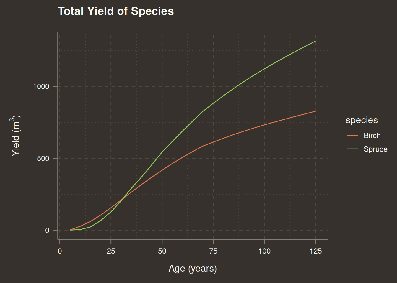
Figure 4 shows that spruce yields more than Birch. This is interesting to see, since it was thinned more times than Birch. Findings like this gives us an insight of the importance of interventions made in the forest.

yield_tbl |> 
  ggplot(aes(age, total_yield, col = species)) +
  geom_line() +
  labs(
    x = "Age (years)",
    y = expression(paste("Yield (", m^{3}, ")")),
    title = "Total Yield of Species"
  )

Figure 4: Total yield of the tree species over time. Spruce has more volume than Birch

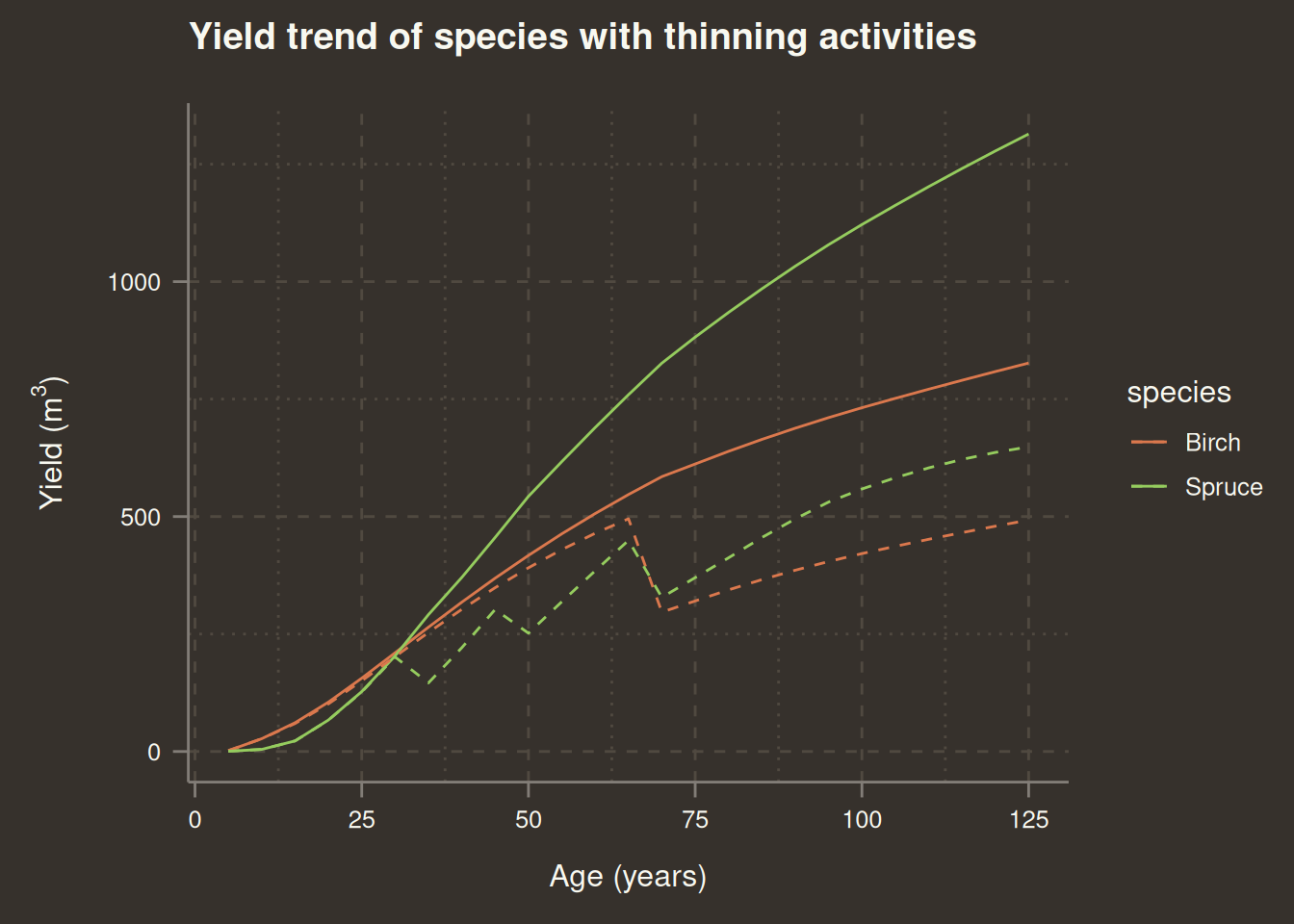
Figure 5 clearly shows this relationship as the yield rate increases for the species after thinning operation.

yield_tbl |> 
  ggplot(
    aes(age, total_yield, col = species)
  ) +
  geom_line() +
  geom_line(aes(age, stand_vol), linetype = 2) +
  labs(
    x = "Age (years)",
    y = expression(paste("Yield (", m^{3}, ")")),
    title = "Yield trend of species with thinning activities"
  )

Figure 5: Total yield of species and their

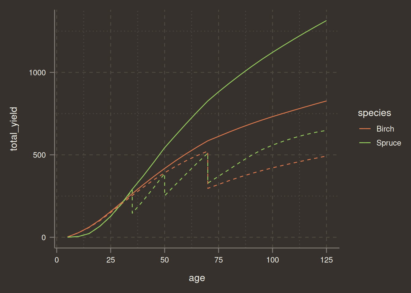
While we have good visuals, Figure 5 can be misleading. What is displayed here is that a thinning operation lasts for more than a year. We will need to correct that, and then we will get a clear read of the thinning intensities.

Correcting the Thinning Age

Usually, the year of harvest or thinning has two volumes and time. The first is the volume before we harvest, and the second is the volume we harvest. They are usually the same, but the time of harvest differs by days or months. Since forestry is a business that involves calculating stand volume over a yearly period of time. It is usually costly and unprofitable to carry out inventory every year; thus, it is carried out between certain periods, 5 to 10 years or more, depending on the management objective and the forest manager’s decision, while we still monitor the stand between such periods. Now we adjust the year of thinning and standing volume to show the age before harvest.

thinning_tbl <- yield_tbl |> 
  filter(harv_vol > 0) |> 
  mutate(
    age = age - 0.01,
    stand_vol = stand_vol + harv_vol
  )

yield_cor_tbl <- yield_tbl |> 
  bind_rows(thinning_tbl) |> 
  arrange(site, age)

head(yield_cor_tbl, 10)

# A tibble: 10 × 14
    site   age species stdens      ba tot_vol stand_vol harv_vol mor_vol
   <dbl> <dbl> <fct>    <dbl>   <dbl>   <dbl>     <dbl>    <dbl>   <dbl>
 1     1   5   Spruce   2019.  0.0834    0.6        0.6       0     0   
 2     1  10   Spruce   1999.  1.75      4.51       4.5       0     0.01
 3     1  15   Spruce   1985.  7.09     22.5       22.5       0     0.03
 4     1  20   Spruce   1970. 15.0      67.0       66.8       0     0.15
 5     1  25   Spruce   1948. 22.4     127.       127.        0     0.64
 6     1  30   Spruce   1922. 29.8     203.       201.        0     1.44
 7     1  35.0 Spruce   1890. 36.9     289.       286.      140.    2.74
 8     1  35   Spruce   1890. 36.9     289.       146.      140.    2.74
 9     1  40   Spruce    843. 25.4     225.       221.        0     4.25
10     1  45   Spruce    826. 32.2     306.       302.        0     3.77
# ℹ 5 more variables: spruce_dgv <dbl>, birch_dgv <dbl>, cum_har <dbl>,
#   cum_mort <dbl>, total_yield <dbl>

yield_cor_tbl |> 
  ggplot(
    aes(age, total_yield, col = species)
  ) +
  geom_line() +
  geom_line(aes(age, stand_vol), linetype = 2)

Heavy or Light?

The definition of what is heavy or not is something that varies depending on the parameter used for thinning, viz basal area or stand density, but for simplicity, stand density will be the parameter used to determine the thinning intensity (check ?@fig-std-dens-trend). Based on the stand density or number of trees removed from the stand, thinning ≤ 25% is regarded as light thinning, 50% regarded as moderate, and > 50% is regarded as heavy thinning (Gonçalves, 2021). Using the thinning intensity or degree formula provided by Gonçalves 2021.

\[𝑅𝑁=𝑁𝑟𝑒𝑚/𝑁𝑡\]

Where - Nrem = Number of trees removed - Nt = Total number of trees

Species	Age	Stand density	Thinning intensity	Light or Heavy?
Spruce	35 and 40	1890.1-842.8	55.4% Heavy
Spruce	50 and 55	816.2/517.6	36.6%	Moderate
Spruce	70 and 75	565.9 - 340.9	39.8%	Moderate
Birch	70 - 75	1465.7 - 785.5	46.4%	Moderate

Conclusion

This thinning experiment highlights how management intensity influences stand development and yield. Spruce consistently outperformed Birch in both total volume and cumulative yield, despite undergoing more thinning interventions. The analysis shows that Birch experienced only one moderate thinning, whereas Spruce had three interventions, ranging from heavy to moderate intensity.

These findings emphasize two key insights for forest managers:

Thinning frequency and intensity matter—they can significantly influence long-term productivity without necessarily reducing yield.

Species-specific responses—Spruce demonstrated resilience and sustained growth after multiple thinnings, suggesting it can better capitalize on reduced competition compared to Birch.

Ultimately, thinning is not just a volume-reduction exercise; when planned correctly, it becomes a strategic tool for enhancing stand quality, maximizing yield, and meeting management objectives over time.