How old is that Possum?

Introduction

This project aims to predict the age of possums collected from three different sites in Australia using linear regression.. The sites are Victoria, New South Wales and Queensland. New South Wales and Queensland are compressed into a single category “Others”. The data is available in the DAAG R package developed by Maindonald, Braun, and Braun (2015).

Cute Possum

The data is having the following properties:

S/N	Variable name	Definition
1.	case	Observation number
2.	site	The site number where the possum was trapped.
3.	Pop	The site as Vic (Victoria) or Other (New South Wales and Queensland)
4.	sex	Gender, either m (male) or f (female).
5.	age	Age of possum
6.	hdlngth	Head length, in mm.
7.	skullw	Skull width, in mm.
8.	totlngth	Total length, in cm.
9.	taill	Tail length, in cm.
10.	footlgth	Foot length in mm
11.	earconch	Ear conch length in mm
12.	eye	distance from medial canthus to lateral canthus of right eye
13.	chest	chest girth (in cm)
14.	belly	belly girth (in cm)

pacman::p_load(tidyverse, GGally, knitr, ggthemr, tidymodels, themis)
ggthemr("grape")

Loading the data

psm <- DAAG::possum |> janitor::clean_names() |> 
  remove_rownames() |> as_tibble()

After getting any data, the first thing to do is trying to understand the data

skimr::skim_without_charts(psm)

Table 1: Summary statistics of possum data

(a)

Name	psm
Number of rows	104
Number of columns	14
_______________________
Column type frequency:
factor	2
numeric	12
________________________
Group variables	None

Variable type: factor

(b)

skim_variable	n_missing	complete_rate	ordered	n_unique	top_counts
pop	0	1	FALSE	2	oth: 58, Vic: 46
sex	0	1	FALSE	2	m: 61, f: 43

Variable type: numeric

(c)

skim_variable	n_missing	complete_rate	mean	sd	p0	p25	p50	p75	p100
case	0	1.00	52.50	30.17	1.0	26.75	52.50	78.25	104.0
site	0	1.00	3.62	2.35	1.0	1.00	3.00	6.00	7.0
age	2	0.98	3.83	1.91	1.0	2.25	3.00	5.00	9.0
hdlngth	0	1.00	92.60	3.57	82.5	90.68	92.80	94.73	103.1
skullw	0	1.00	56.88	3.11	50.0	54.98	56.35	58.10	68.6
totlngth	0	1.00	87.09	4.31	75.0	84.00	88.00	90.00	96.5
taill	0	1.00	37.01	1.96	32.0	35.88	37.00	38.00	43.0
footlgth	1	0.99	68.46	4.40	60.3	64.60	68.00	72.50	77.9
earconch	0	1.00	48.13	4.11	40.3	44.80	46.80	52.00	56.2
eye	0	1.00	15.05	1.05	12.8	14.40	14.90	15.72	17.8
chest	0	1.00	27.00	2.05	22.0	25.50	27.00	28.00	32.0
belly	0	1.00	32.59	2.76	25.0	31.00	32.50	34.12	40.0

Table 1 (a) shows that data was collected on 104 possum’s. There are 2 categorical variables, pop and sex, but this should be three as site should also be a categorical variable (check below to see transformation of this variable). The case variable is not needed and can be removed. There are missing data in age and footlgth variables, Table 1 (b). We can remove this missing data points as it’s not a lot, Figure 1.

visdat::vis_miss(psm)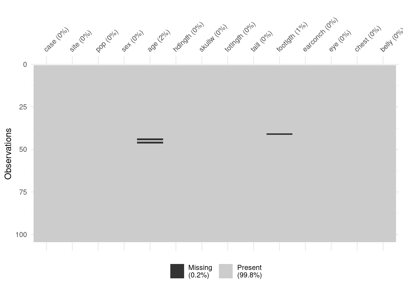

Figure 1

psm <- psm |> 
  drop_na() |> 
  select(-case) |> 
  mutate(
    site = factor(
      site, 
      levels= 1:7,
      labels = c("Cambarville", "Bellbird", "Whian Whian",
                "Byrangery", "Conondale", "Allyn River", "Bulburin")
    )
  )

Exploratory Data Analysis

To understand the data, we do an EDA for targets and predictors.

Univariate Analysis - Target

psm |> 
  summarize(
    median_age = median(age),
    mean_age = round(mean(age), 2),
    minimum_age = min(age),
    maximum_age = max(age)
  ) |> kable(
    col.names = c("Median", "Mean", "Min", "Max"),
    align = "lccr",
    caption = "Measure of Central Tendency for Age"
  )

Table 2: Descriptive Statistics for Possum Age

Measure of Central Tendency for Age

Median	Mean	Min	Max
3	3.82	1	9

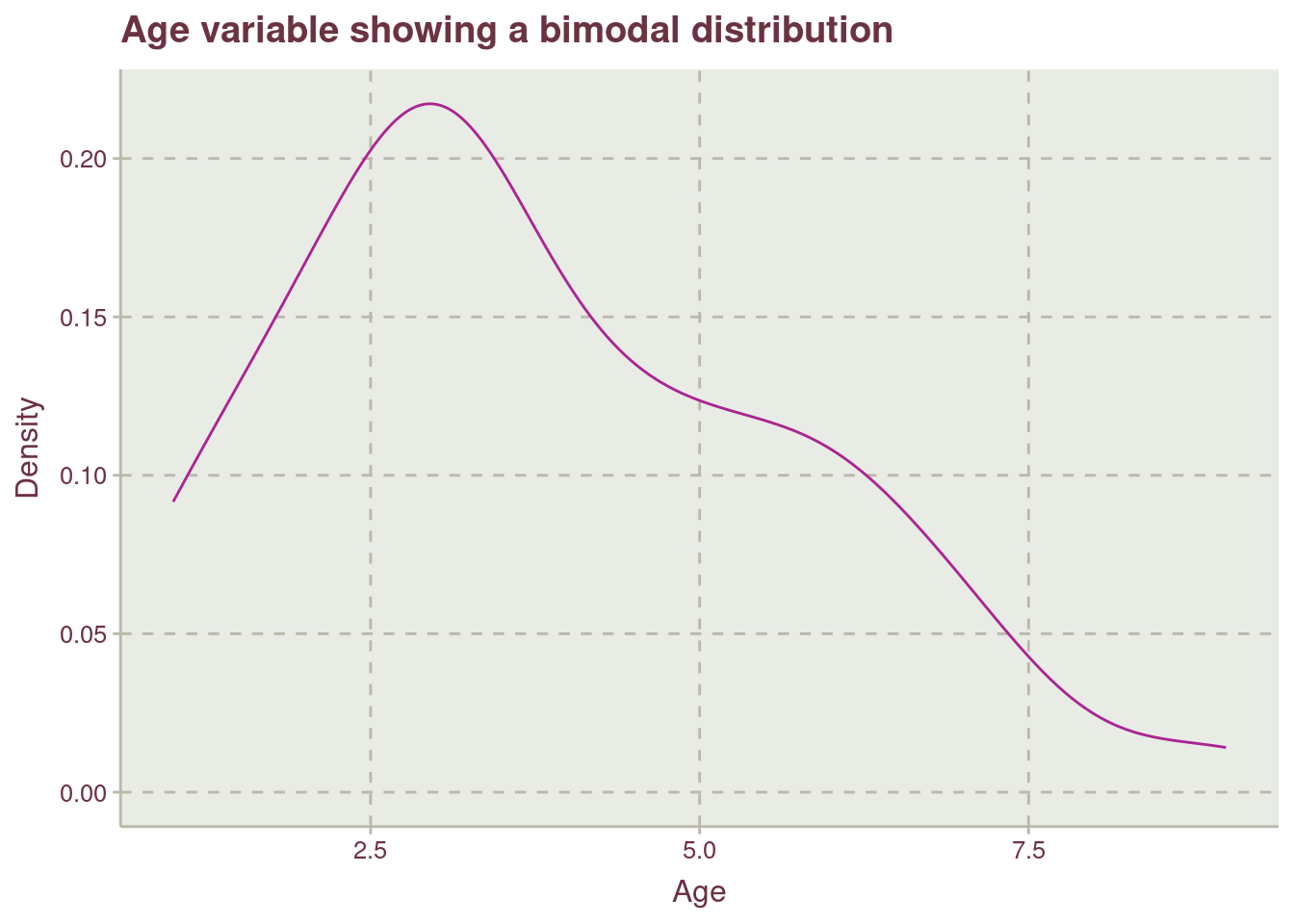
Table 2 shows a spread mean and median value for age which might indicates that the distribution is skewed or bimodal, see Figure 2.

psm |> 
  ggplot(aes(age)) +
  geom_density(col = "#ab2493") +
  labs(
    x = "Age",
    y = "Density",
    title = "Age variable showing a bimodal distribution"
  )

Figure 2: Distribution of Age variable

Univariate Analysis of Features

Factors

Regions and Sites (Trap Locations)

psm |> 
  mutate(
    pop = case_when(
      pop == "Vic" ~ "Victoria",
      .default = "Others"
    )
  ) |> 
  ggplot(aes(pop)) +
  geom_bar(fill = "cadetblue4") +
  expand_limits(y = c(0, 70)) +
  labs(
    x = "Population",
    y = "Frequency",
    title = "Population of Registered Possums According to Regions"
  ) +
  theme(plot.title = element_text(face = "bold", hjust = .5))

psm |> 
  count(site) |> 
  arrange(n) |> 
  ggplot(aes(n, fct_reorder(site, n))) +
  geom_bar(
    stat = "identity",
    fill = "coral2"
  ) +
  labs(
    y = "Sites",
    x = "Count",
    title = "Population of Registered Possums According to Sites"
  ) +
  theme(
    plot.title = element_text(face = "bold", hjust = .5)
  )

(a)

(b)

Figure 3: Registered Possum Population Record

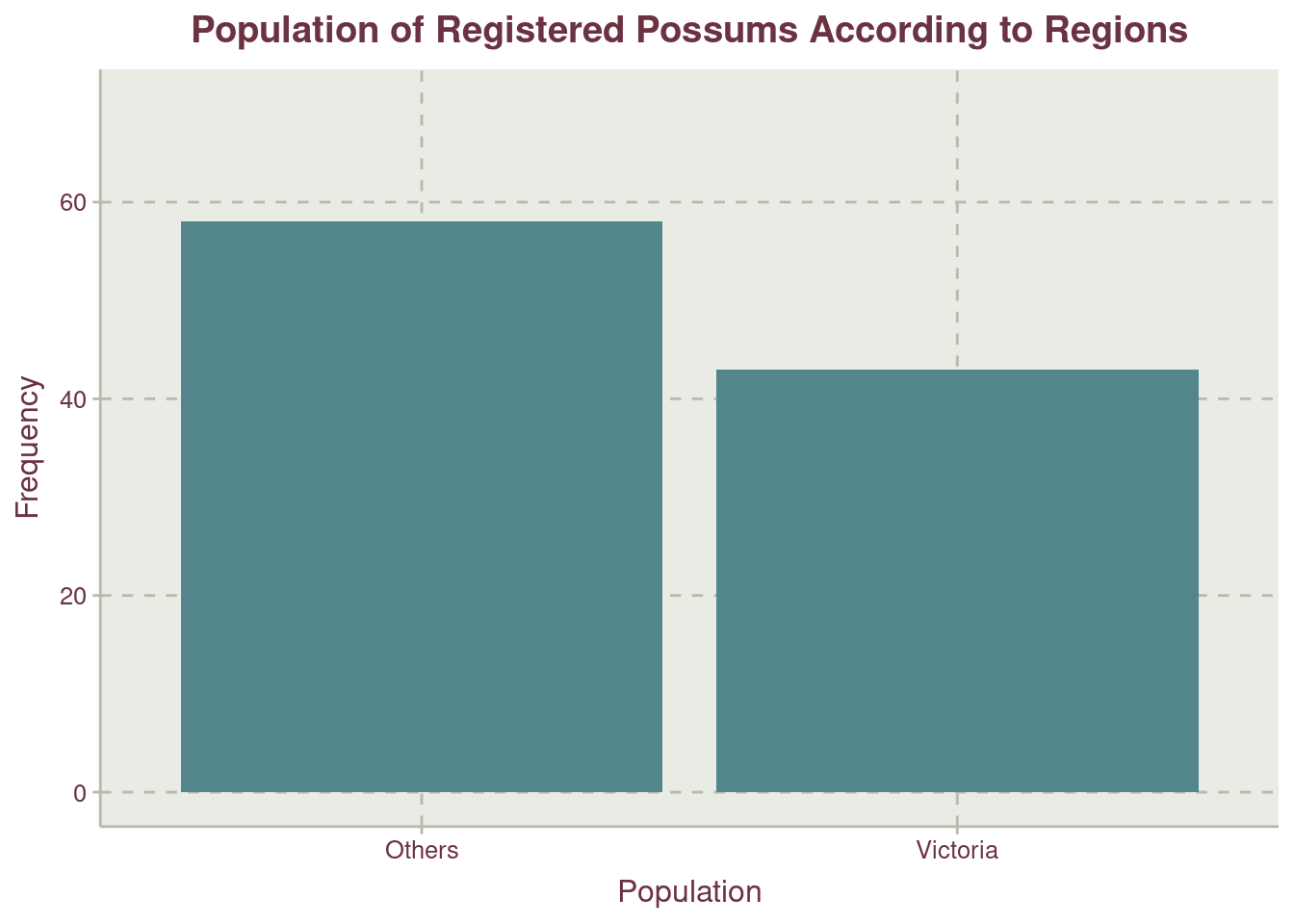
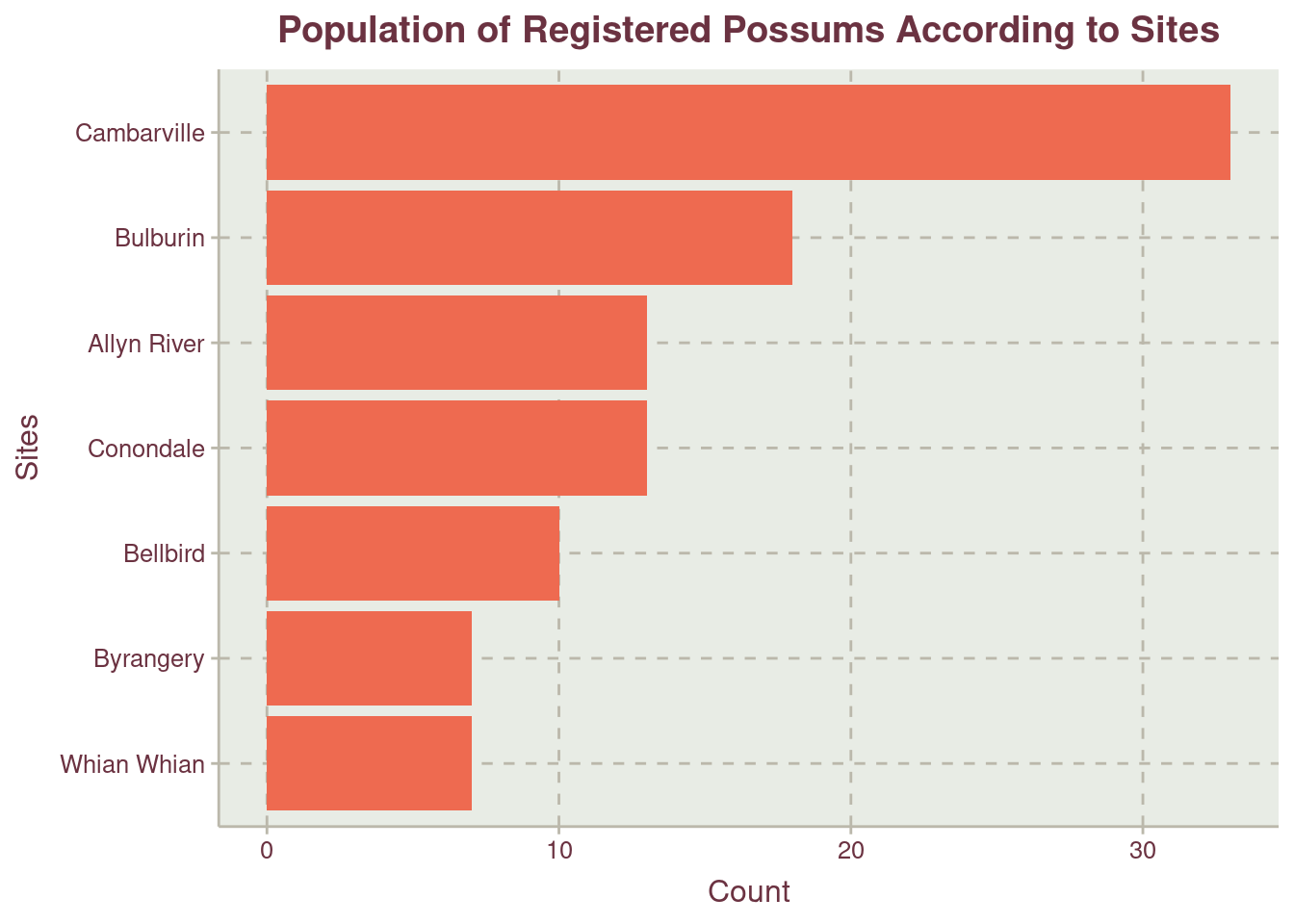
More possums were recorded at the region labelled Other Figure 3. We should recall that Other is the combination of records from New South Wales and Queensland. For the sites where trap where placed within the regions, Cambarville have the highest record of possums with more than half the second site, Bulburin.

Numerical Variables

psm_long <- psm |> 
  pivot_longer(
    cols = hdlngth:belly,
    names_to = "variables",
    values_to = "values"
  )

psm_long |> 
  summarize(
    .by = variables,
    mean = mean(values),
    median = median(values),
    minimum = min(values),
    maximum = max(values)
  ) |> 
  kable(
    col.names = c("Variable", "Mean", "Median", "Minimum", "Maximum"),
    align = "lcccr"
  )

Table 3: Measure of Central Tendency for Numerical Variable

Variable	Mean	Median	Minimum	Maximum
hdlngth	92.73069	92.9	82.5	103.1
skullw	56.96040	56.4	50.0	68.6
totlngth	87.26931	88.0	75.0	96.5
taill	37.04951	37.0	32.0	43.0
footlgth	68.39802	67.9	60.3	77.9
earconch	48.13366	46.8	41.3	56.2
eye	15.05049	14.9	12.8	17.8
chest	27.06436	27.0	22.0	32.0
belly	32.63861	32.5	25.0	40.0

Table 3 shows the measure of central tendency. The difference between median and mean is minimal indicating a normal distribution.

additional_colors <- c("#af4242", "#535364", "#FFC300")
set_swatch(c(unique(swatch()), additional_colors))

psm_long |> 
  ggplot(aes(values, col = variables)) +
  geom_density() +
  scale_color_discrete() +
  facet_wrap(~variables, scales = "free") +
  theme(legend.position = "none")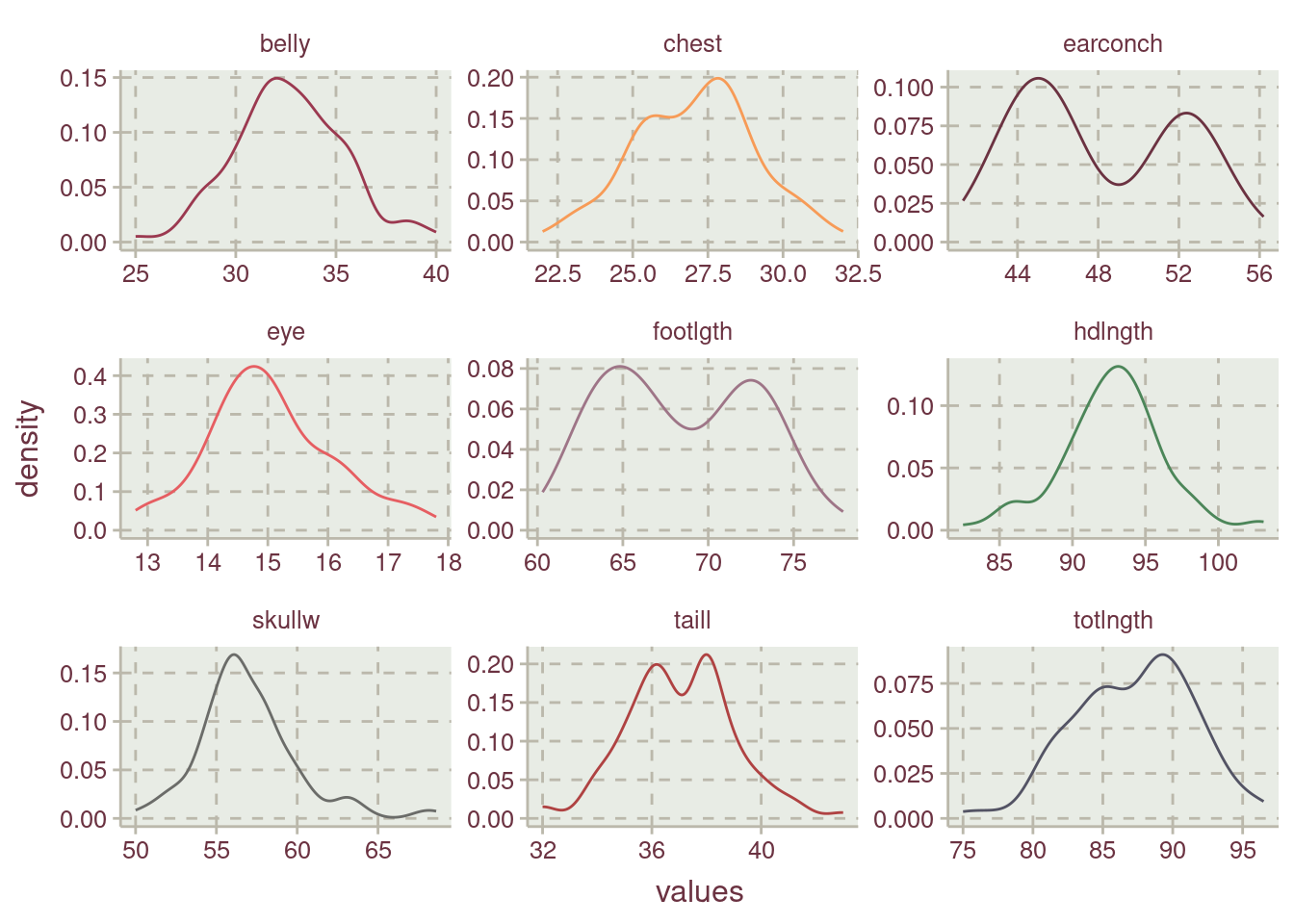

Figure 4: Numerical variable distribution

All the numerical variables are normally distributed Figure 4. earconch, footlgth, taill, and totlngth are bimodals.

Multivariate Analysis

psm |>
  mutate(
    pop = case_when(
      pop == "Vic" ~ "Victoria",
      .default = "Others"
    )
  ) |> 
  ggplot(aes(site, age, fill = pop, col = "#000")) +
  geom_violin(inherit.aes = FALSE, aes(site, age)) +
  geom_boxplot(position = "dodge", width = .2) +
  geom_jitter(size = .5) +
  facet_wrap(~pop, scales = "free") +
  coord_flip() +
  theme(legend.position = "none")

Warning: The `scale_name` argument of `discrete_scale()` is deprecated as of ggplot2
3.5.0.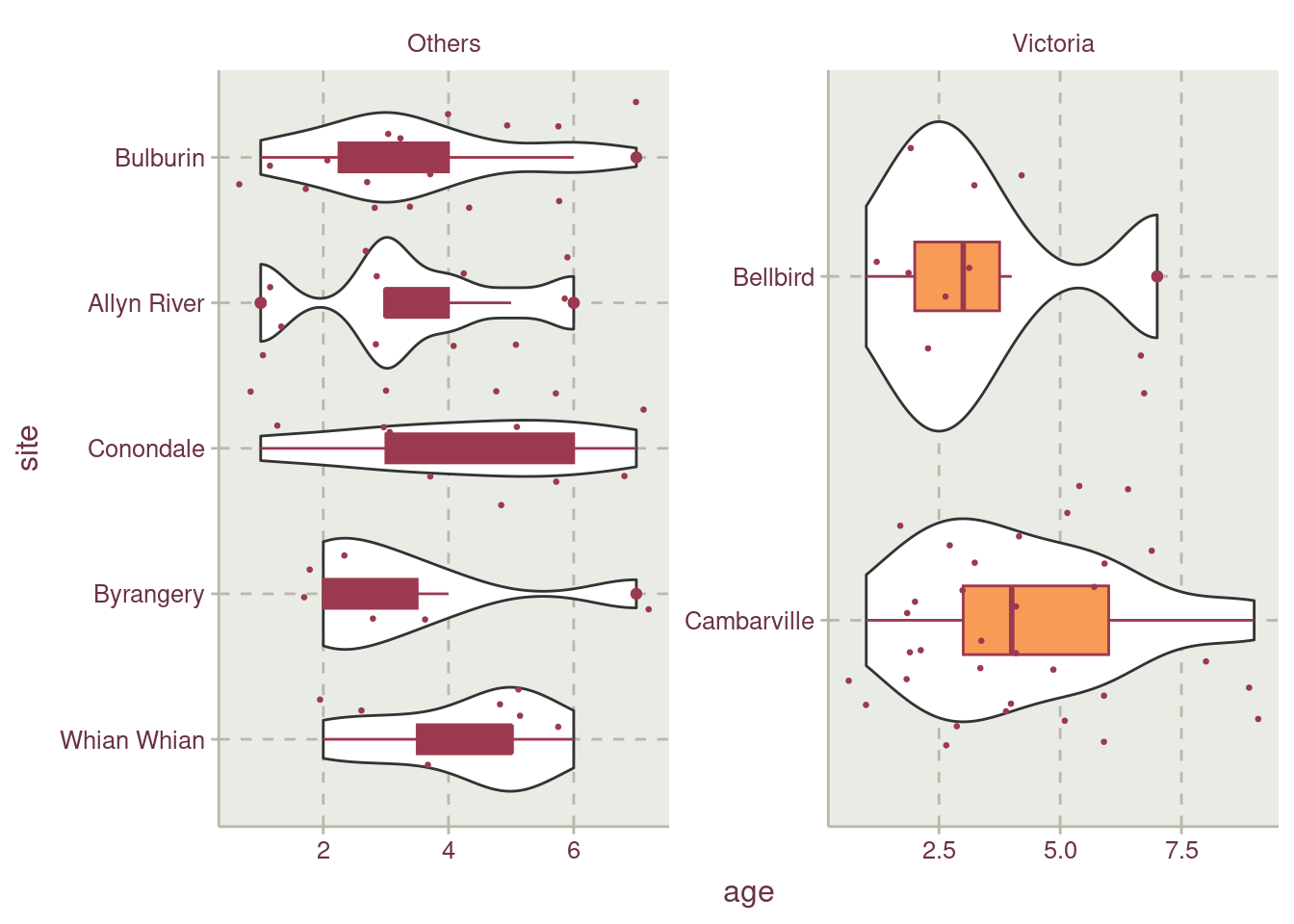

Correlation Matrix

ggcorr(
  psm,
  geom = "text",
  low = "#219123",
  mid = "#e09263",
  high = "#8f0123"
)

Figure 5: Correlation Matrix

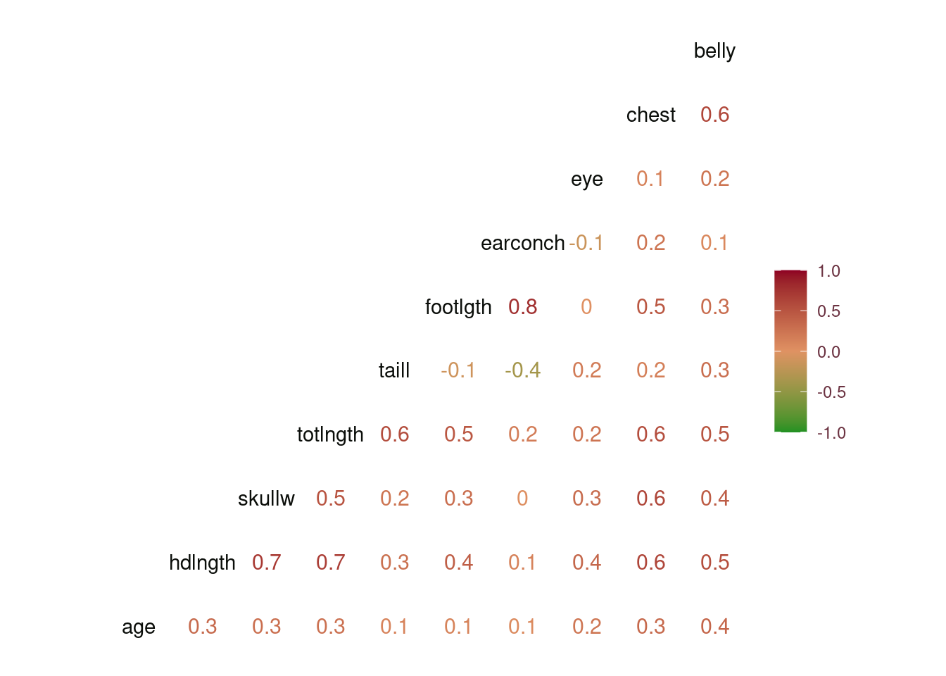
The correlation of the variables to age is low with the maximum correlation being with belly, Figure 5. However, there’s high correlation between the predictors and to prevent collinearity we could consider employing Principal Component Analysis to transform correlated predictors to uncorrelated predictor. More information on the relationships existing between the variables can be seen in Figure 6.

ggpairs(psm)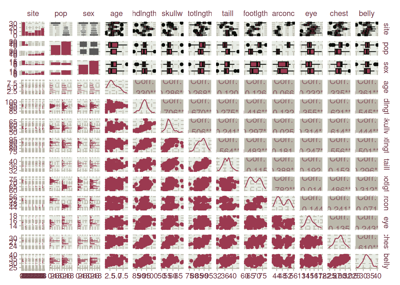

Figure 6: Generalized pairs plot

Modeling

Data Sharing

Figure 2 shows how older possums from age 8 to 9 are not well represented in the data. A stratified data sharing technique will be employed to account for less represented age data point.

set.seed(124)
psm_split <- initial_split(psm, prop = .75, strata = age)
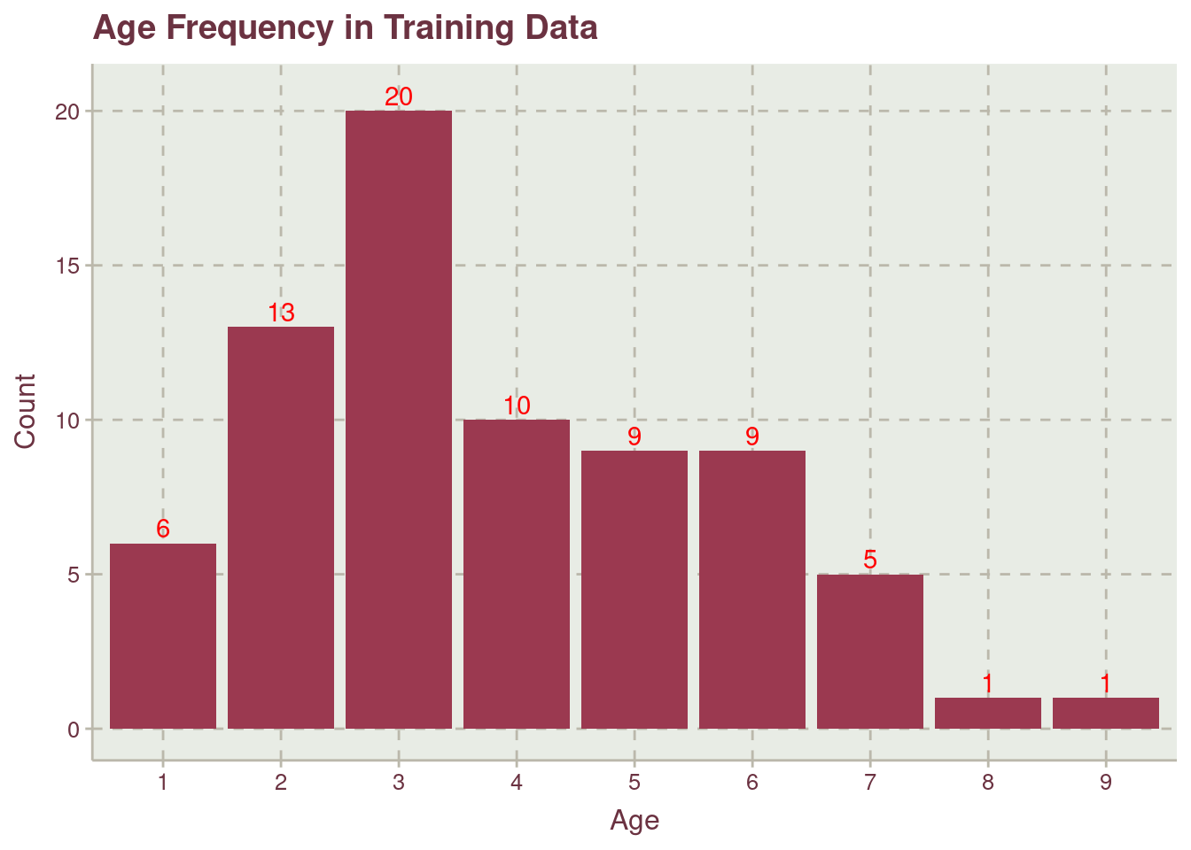
psm_train <- training(psm_split)

If we check Figure 7, possums that are 8 and 9 years old are represented.

psm_train |> 
  count(age) |> 
  ggplot(aes(factor(age), n)) +
  geom_col() +
  geom_text(
    aes(label = n),
    nudge_y = .5,
    col = "red"
  ) +
  labs(
    x = "Age",
    y = "Count",
    title = "Age Frequency in Training Data"
  )

Figure 7: Age data point frequency in training data

To prevent data leaking, the data will be resampled to have a validation-training data in 10 folds using the k-folds resampling.

set.seed(124)
psm_folds <- vfold_cv(psm_train, v = 10)

Model Specification

We will use linear regression to predict the age of possums

lm_spec <- linear_reg() |> 
  set_engine("lm")
lm_spec |> translate()

Linear Regression Model Specification (regression)

Computational engine: lm 

Model fit template:
stats::lm(formula = missing_arg(), data = missing_arg(), weights = missing_arg())

Feature engineering

Three preprocessing will be added to formular specification. These are:

• Normalizing, centering and scaling numerical variables
• PCA to reduce collinearity between numeric variables
• Creating dummy variables for categorical data.

These preprocesses are added as presented down to the last step which is creating dummy variables for categorical data.

psm_rec_1 <- recipe(age ~ ., data = psm_train)

psm_rec_2 <- psm_rec_1 |> 
  step_normalize(all_numeric_predictors()) |> 
  step_center(all_numeric_predictors()) |> 
  step_scale(all_numeric_predictors())

psm_rec_3 <- psm_rec_2 |> 
  step_pca(all_numeric_predictors())

psm_rec_4 <- psm_rec_3 |>
  step_dummy(all_factor_predictors()) 

The result from applying the whole steps is shown in Table 4

psm_rec_4 |> 
  prep() |> 
  juice() |> 
  head() |> 
  kable()

Table 4: Data look after preprocessing

age	PC1	PC2	PC3	PC4	PC5	site_Bellbird	site_Whian.Whian	site_Byrangery	site_Conondale	site_Allyn.River	site_Bulburin	pop_other	sex_m
2	-0.0683403	-1.343005	0.1629385	-0.3007284	-0.5391333	0	0	0	0	0	0	0	0
1	0.5255119	-2.047798	-0.8395109	0.1766334	-0.0667790	0	0	0	0	0	0	0	0
2	0.5932377	-1.959162	0.3740650	0.6887651	0.0693626	0	0	0	0	0	0	0	1
2	-0.2120375	-2.211136	1.7088223	-0.3387357	-0.0931182	0	0	0	0	0	0	0	1
2	-2.7210452	-1.389487	0.2290110	0.7561382	1.2385934	0	0	0	0	0	0	0	0
2	-1.6707158	-1.652564	0.3608677	-0.3541424	-0.3539676	0	0	0	0	0	0	0	0

The numerical predictors has been reduced to 5 variables.

Model Workflow

psm_wf_set <- workflow_set(
  preproc = list(
    "formula" = psm_rec_1,
    "normalized" = psm_rec_2, 
    "pca" = psm_rec_3,
    "dummy" = psm_rec_4
  ),
  models = list("ols" = lm_spec),
  cross = TRUE
)

psm_wf_set

# A workflow set/tibble: 4 × 4
  wflow_id       info             option    result    
  <chr>          <list>           <list>    <list>    
1 formula_ols    <tibble [1 × 4]> <opts[0]> <list [0]>
2 normalized_ols <tibble [1 × 4]> <opts[0]> <list [0]>
3 pca_ols        <tibble [1 × 4]> <opts[0]> <list [0]>
4 dummy_ols      <tibble [1 × 4]> <opts[0]> <list [0]>

Fitting the model

psm_mod <- psm_wf_set |> 
  workflow_map(
    "fit_resamples",
    resamples = psm_folds,
    seed = 124
)

collect_metrics(psm_mod) |> kable()

Table 5: Model metric

wflow_id	.config	preproc	model	.metric	.estimator	mean	n	std_err
formula_ols	Preprocessor1_Model1	recipe	linear_reg	rmse	standard	1.7863370	10	0.1001647
formula_ols	Preprocessor1_Model1	recipe	linear_reg	rsq	standard	0.2506679	10	0.0642785
normalized_ols	Preprocessor1_Model1	recipe	linear_reg	rmse	standard	1.7863370	10	0.1001647
normalized_ols	Preprocessor1_Model1	recipe	linear_reg	rsq	standard	0.2506679	10	0.0642785
pca_ols	Preprocessor1_Model1	recipe	linear_reg	rmse	standard	1.7590867	10	0.1122277
pca_ols	Preprocessor1_Model1	recipe	linear_reg	rsq	standard	0.1970622	10	0.0555754
dummy_ols	Preprocessor1_Model1	recipe	linear_reg	rmse	standard	1.7590867	10	0.1122277
dummy_ols	Preprocessor1_Model1	recipe	linear_reg	rsq	standard	0.1970622	10	0.0555754

Table 5 shows no difference in the model between dummy_ols and pca_ols which is different from using the formula without preprocessing, formula_ols and normalized_ols. This presented visually in Figure 8

collect_metrics(psm_mod) |> 
  filter(.metric == "rmse") |> 
  select(wflow_id, mean, std_err) |> 
  mutate(
    ymax = mean + std_err,
    ymin = mean - std_err
  ) |> 
  ggplot(aes(wflow_id, mean, col = wflow_id)) +
  geom_pointrange(aes(ymin = ymin, ymax =ymax)) +
  labs(
    x = "Preproc",
    title = "RMSE of Possum Linear Regression Model for 3 Preprocessor"
  ) +
  theme(legend.position = "none")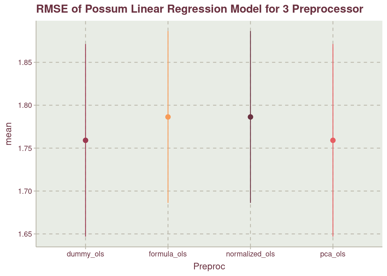

Figure 8: Model evaluation using RMSE for each preprocessor

We can use either of pca_ols or dummy_ols as they have the lowest mean.

psm_pca_mod <- psm_mod |> 
  extract_workflow(id = "pca_ols")

psm_pca_mod 

══ Workflow ════════════════════════════════════════════════════════════════════
Preprocessor: Recipe
Model: linear_reg()

── Preprocessor ────────────────────────────────────────────────────────────────
4 Recipe Steps

• step_normalize()
• step_center()
• step_scale()
• step_pca()

── Model ───────────────────────────────────────────────────────────────────────
Linear Regression Model Specification (regression)

Computational engine: lm 

psm_model <- last_fit(
  psm_pca_mod,
  split = psm_split
)

psm_model |> 
  collect_predictions() |> 
  select("prediction" =.pred, age) |> 
  mutate(
    prediction = ceiling(prediction),
    residual = age - prediction
  ) |> 
  ggplot(
    aes(age, residual)
  ) +
  geom_point() +
  geom_hline(aes(yintercept = 0), col = "gray3") +
  ggtitle("Residual")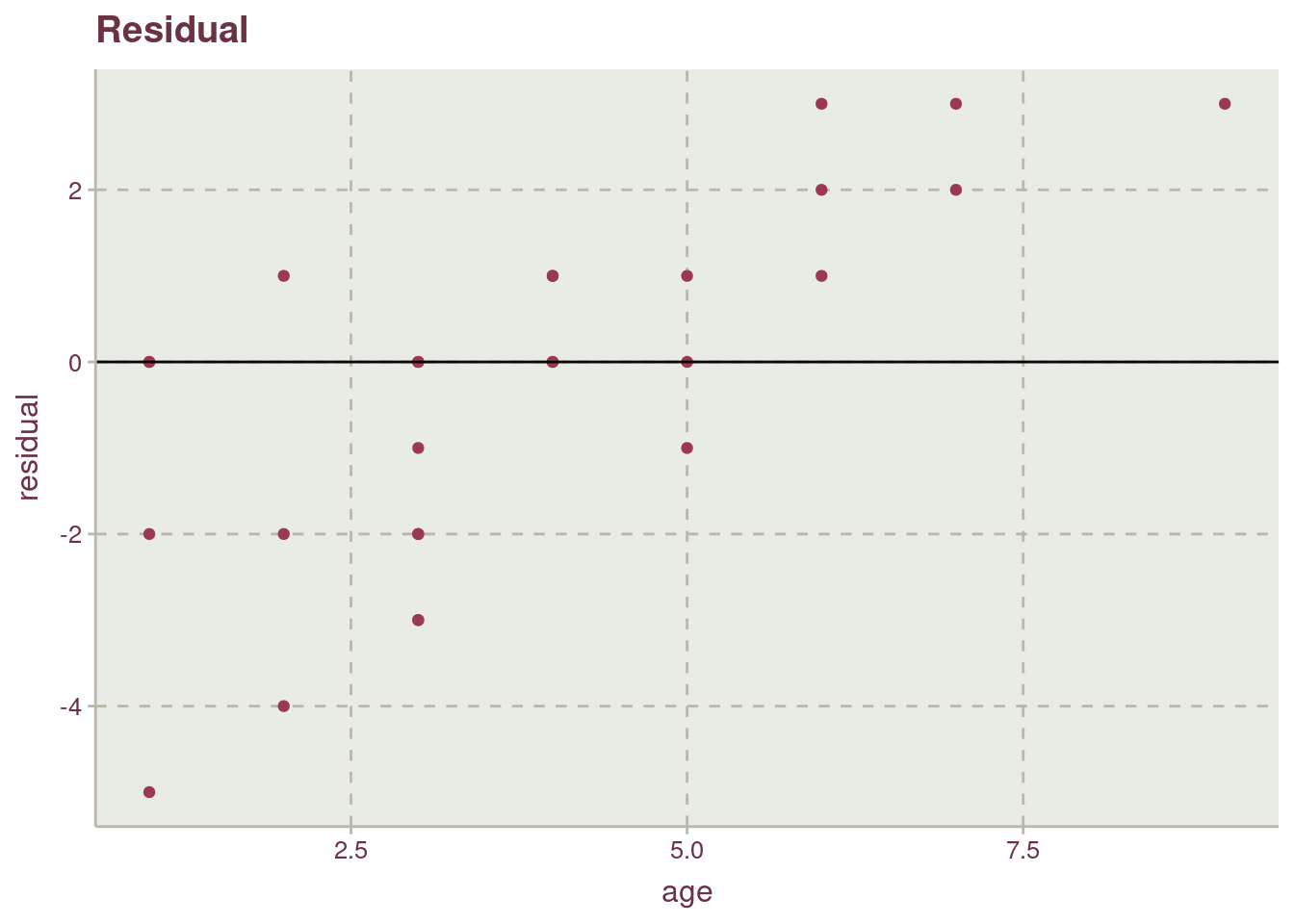

While the points are fairly distributed along the y axis and x axis, the effect of having little representative from the population for old-aged possum, age 9 and 8 can be see. The lack of points on the lower-right side of the plot is a good of indication.

Feature Importance

The features contributing the most to the model are shown in Figure 9

psm_model |>
  extract_fit_parsnip() |> 
  vip::vip(
    num_features = 10,
    geom = "col"
  ) +
  ggtitle("Feature Importance")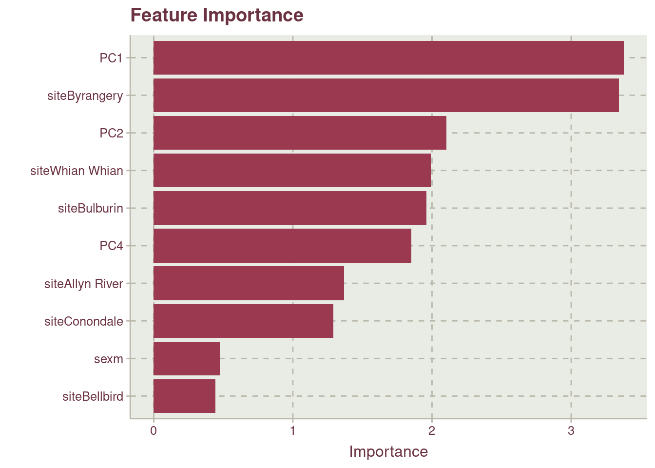

Figure 9: PC1, and Byrangery sites are the most important variables.

Summary

While this a good use of linear regression, the robustness of the model would have been helped if underrepresented data points are available. By the time of writing this blog post, the author with intentions to use only SLR is having no feature engineering method to account for the age variable that has been discretized. A resampling technique such as Monte Carlo or bootstrapping is an approach that could help with the model rather than the use of k-fold resampling method.

References

Maindonald, John H, W John Braun, and Maintainer W John Braun. 2015. “Package ‘DAAG’.” Data Analysis and Graphics Data and Functions.