Mapping the Urban Forest: Exploring Tree Data in Salinas, California 🌳

Urban trees are more than just greenery along our streets—they provide shade, improve air quality, and shape the character of a city. Thanks to open data initiatives, we can analyze and visualize tree inventories to better understand the composition and health of urban forests.

In this post, we’ll walk through an exploration of the City of Salinas, California’s tree inventory dataset, using Python tools like GeoPandas, Matplotlib, and Contextily to map and categorize the trees.

First we will import the packages used in this post. We can use either uv, pip, conda

import pandas as pd
import geopandas as gpd
import contextily as cx
from janitor import drop_constant_columns
import matplotlib.pyplot as plt

Data Importation

The data used in this analysis was downloaded from opendatasoft. We start by loading the tree inventory GeoJSON file with geopandas. Since many datasets contain placeholder values like N/A, we replace them with pandas actual NA value–pd.NA. To simplify the dataset, we also remove constant columns (columns with the same value for all rows).

inv_tbl_raw = gpd.read_file("data/tree-inventory-cityofsalinas.geojson")
inv_tbl = inv_tbl_raw.replace("N/A", pd.NA).drop_constant_columns()
inv_tbl.head()

Table 1: Data preview

	objectid	id	uniqueid	address	street	onstr	fromstr	tostr	side	site	...	spacesize	subzone	parkquad	zone	district	stmpvcnt	globalid	suffix	geo_point_2d	geometry
0	32031	30339	IH 20140709074052	283	CHAPARRAL ST	MARYAL DR	DEADEND	CHAPARRAL ST	Right	1	...	10.0	<NA>	<NA>	<NA>	4	No	{FFA7B88F-19F4-4FA2-9008-C6954AA0EB05}	None	{ "lon": -121.64605930227704, "lat": 36.703282...	POINT (-121.64606 36.70328)
1	32070	2496	BS 20140424130746	183	DENNIS AV	DENNIS AV	MIAMI ST	TAMPA ST	Front	1	...	5.0	<NA>	<NA>	<NA>	2	No	{E2350667-2941-42E7-A09B-A90151C81680}	None	{ "lon": -121.60828225058304, "lat": 36.675840...	POINT (-121.60828 36.67584)
2	32084	8825	BS 20140516133448	1271	MORENO DR	TOWT ST	MORENO WY	PASEO GRANDE	Rear	5	...	6.0	<NA>	<NA>	North/East Maintenance District	1	No	{37810329-E153-4E5B-9AFE-6F9CFD3C60BD}	None	{ "lon": -121.60240705321014, "lat": 36.687945...	POINT (-121.60241 36.68795)
3	32085	8833	BS 20140516134752	1255	MORENO DR	TOWT ST	MORENO WY	PASEO GRANDE	Rear	1	...	7.0	<NA>	<NA>	North/East Maintenance District	1	No	{C56D21E6-D6EA-4F76-941C-5C8CEBC53826}	None	{ "lon": -121.6030825123258, "lat": 36.6876225...	POINT (-121.60308 36.68762)
4	32092	9077	BS 20140519122755	1252	MORENO DR	MORENO DR	CAMARILLO CT	CAYUCOS CIR	Front	1	...	10.0	<NA>	<NA>	North/East Maintenance District	1	No	{DBDAD81C-8515-4AD0-A5EA-39291339AADD}	None	{ "lon": -121.60290566856168, "lat": 36.687211...	POINT (-121.60291 36.68721)

5 rows × 35 columns

We have interesting variables available in the dataset, but, we do not need all.

inv_tbl.columns

Index(['objectid', 'id', 'uniqueid', 'address', 'street', 'onstr', 'fromstr',
       'tostr', 'side', 'site', 'spp', 'dbh', 'stems', 'height', 'width',
       'condstruc', 'condcrwn', 'cond', 'ohutility', 'klir', 'inspect',
       'hdscape', 'vsiblty', 'sound', 'grow', 'spacesize', 'subzone',
       'parkquad', 'zone', 'district', 'stmpvcnt', 'globalid', 'suffix',
       'geo_point_2d', 'geometry'],
      dtype='object')

We’ll only make use of spp, dbh, geometry, and cond .

retain_col = [
    "spp", "dbh",
    "stems", "height", 
    "width", "cond", 
    "grow","geometry"
]
inv_tbl = inv_tbl.loc[:, retain_col]
inv_tbl.head()

Table 2: Data retained

	spp	dbh	stems	height	width	cond	grow	geometry
0	Fraxinus spp.	1.0	1.0	0 to 10	0 to 10	<NA>	Tree Lawn	POINT (-121.64606 36.70328)
1	Fraxinus oxycarpa	7.0	1.0	21 to 30	21 to 30	Fair	Parkway	POINT (-121.60828 36.67584)
2	Pyrus calleryana	10.0	1.0	21 to 30	21 to 30	Good	Back Up	POINT (-121.60241 36.68795)
3	Celtis sinensis	11.0	1.0	21 to 30	21 to 30	Fair	Back Up	POINT (-121.60308 36.68762)
4	Quercus ilex	11.0	1.0	21 to 30	21 to 30	Good	Tree Lawn	POINT (-121.60291 36.68721)

Table 2 shows the retained columns. The data is currently using the WGS 84 Geographic coordinate reference system.

inv_tbl.crs

<Geographic 2D CRS: EPSG:4326>
Name: WGS 84
Axis Info [ellipsoidal]:
- Lat[north]: Geodetic latitude (degree)
- Lon[east]: Geodetic longitude (degree)
Area of Use:
- name: World.
- bounds: (-180.0, -90.0, 180.0, 90.0)
Datum: World Geodetic System 1984 ensemble
- Ellipsoid: WGS 84
- Prime Meridian: Greenwich

Mapping All Trees

Let’s take a quick view of how the trees are planted in Salinas. We will convert to a mercator projector to work well with contextily.

inv_tbl = inv_tbl.to_crs(epsg=3857)

fig, ax = plt.subplots(figsize=(10, 6))
inv_tbl.plot(
    ax=ax, 
    color="red", 
    alpha=0.4, 
    markersize=2
)
cx.add_basemap(ax, source=cx.providers.OpenTopoMap)
plt.axis("off")
plt.tight_layout()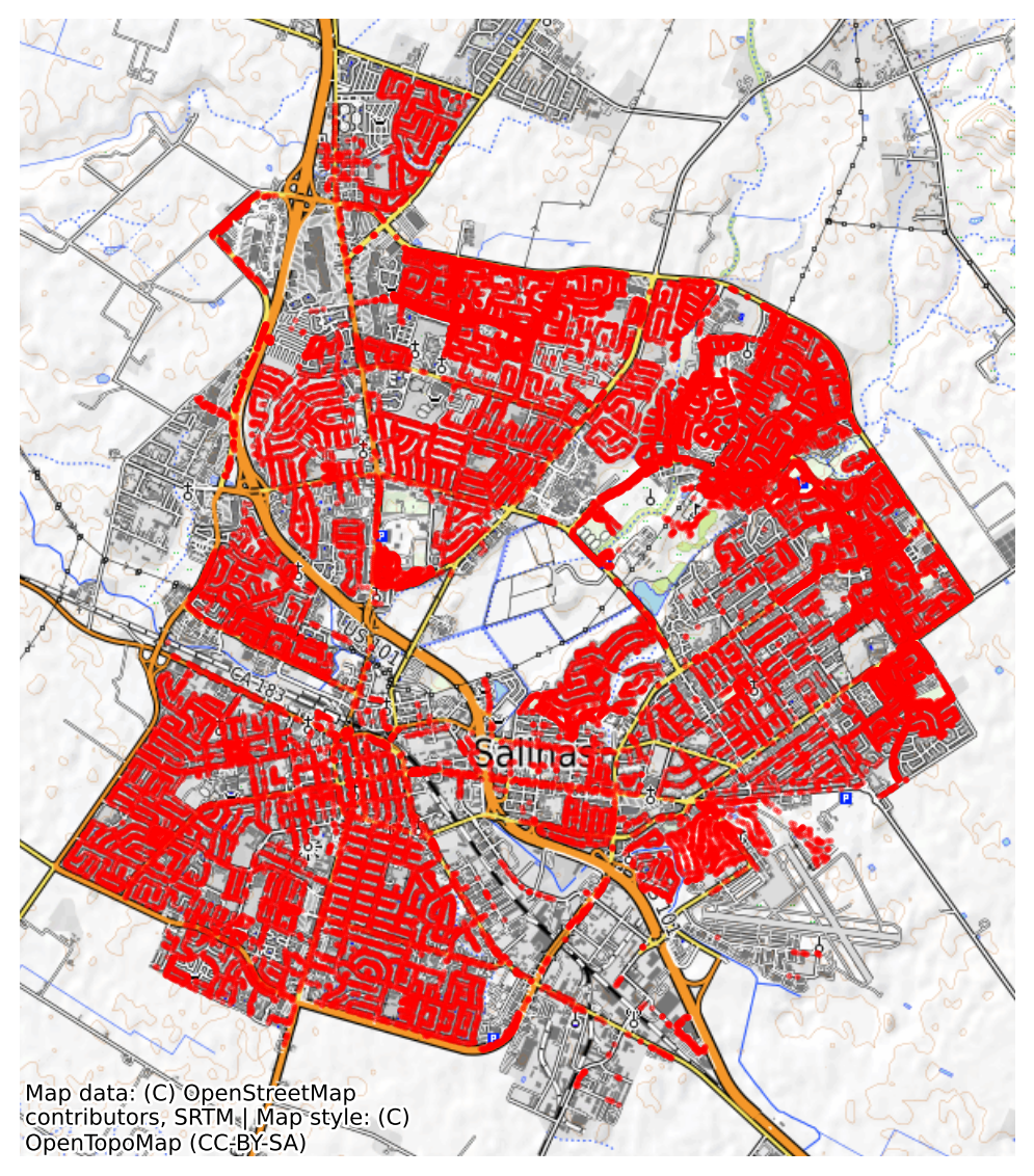

Figure 1: Tree distribution across Salinas. Trees are the red dots

Figure 1 gives us a city-wide snapshot of tree distribution in Salinas and we can tell that Salinas is quite green.

inv_tbl.explore(
    column="grow",
    categorical=True, 
)

Make this Notebook Trusted to load map: File -> Trust Notebook

Figure 2: Tree distribution according to space in Salinas

The overwhelming majority of trees in Salinas grow in parkways and tree lawns, reflecting the city’s street-tree planting strategy. Fewer trees are in medians, parking lot islands, or raised planters, where space and soil volume are more constrained. Very few trees are in unmaintained areas, which makes sense since street tree programs usually focus on maintained urban spaces.

grow_counts = (
    inv_tbl.groupby("grow")["height"]
    .value_counts()
    .unstack(fill_value=0)
)

grow_counts["total"] = grow_counts.sum(axis=1)
grow_counts = grow_counts.sort_values("total", ascending = False).drop(columns = "total")

fig, ax = plt.subplots(figsize=(12, 6))
grow_counts.plot(
    kind="bar",
    ax=ax,
    stacked=False,
    alpha=0.8,
    fontsize=8,
    colormap="tab20",
    edgecolor="#666666",
    legend=True,
    linewidth=0.2
)
ax.set_xlabel("Growing Space", fontsize=10)
ax.set_ylabel("Number of Trees", fontsize=10)
ax.set_title(
    label="Distribution of Trees by Growing Space and Height Category in Salinas", 
    fontsize=13, 
    fontweight="bold"
)
plt.xticks(rotation=40, ha="right")
ax.legend(
    title = "Height",
    bbox_to_anchor=(1.02, 1),
    loc="upper left",
    fontsize=8,
    title_fontsize=10
)
ax.grid(axis="y", linestyle="--", alpha=0.6)
plt.tight_layout()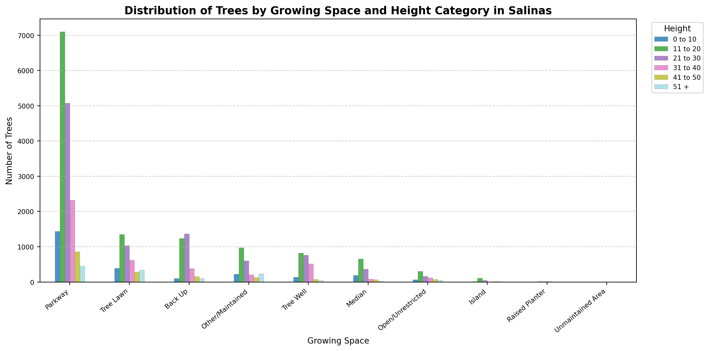

Figure 3: Most trees in Salinas are planted in parkways and tree lawns, with fewer in medians, islands, and planters

Figure 3 further confirms what is suspected by Figure 2. Tree Lawn, Other/Maintained and Backup Seems to possess a large number of tall trees given their number compare to Parkway trees.

Common Species

Liquidambar styraciflua - Source:picry.com

While we have a lot of trees, not all all species are equally represented, Table 3 shows species count.

inv_tbl["spp"].value_counts(ascending=False).head(20)

Table 3: Count of Trees by Species

spp
Liquidambar styraciflua                3147
Pyrus calleryana                       3033
Platanus X acerifolia                  2198
Prunus cerasifera var. atropurpurea    1751
Magnolia grandiflora                   1735
Stump                                  1447
Quercus agrifolia                      1207
Celtis sinensis                        1145
Fraxinus oxycarpa                       982
Cinnamomum camphora                     803
Pyrus kawakamii                         779
Quercus ilex                            694
Prunus serrulata                        642
Maytenus boaria                         615
Sequoia sempervirens                    509
Pinus canariensis                       471
Zelkova serrata                         413
Geijera parviflora                      410
Vacant site, small                      373
Gleditsia triacanthos                   370
Name: count, dtype: int64

To focus on the most common ones, we count species and filter for those with at least 1,000 occurrences, see Table 4.

species_count = inv_tbl["spp"].value_counts()
common_species = species_count[species_count >= 1000].index
common_trees = inv_tbl[inv_tbl["spp"].isin(common_species)]

common_trees["spp"].value_counts()

Table 4: Common trban tree species in Salinas

spp
Liquidambar styraciflua                3147
Pyrus calleryana                       3033
Platanus X acerifolia                  2198
Prunus cerasifera var. atropurpurea    1751
Magnolia grandiflora                   1735
Stump                                  1447
Quercus agrifolia                      1207
Celtis sinensis                        1145
Name: count, dtype: int64

We can plot them on a OpenStreetMap Mapnik basemap.

fig, ax = plt.subplots(figsize=(12, 6))

common_trees.plot(
    ax=ax,
    column="spp",
    categorical=True,
    legend=True,
    markersize=1.5
)
cx.add_basemap(ax, source=cx.providers.OpenStreetMap.Mapnik)
plt.title(
    "Common Tree Species in Salinas, California", 
    fontsize=12, 
    fontweight="bold"
)
plt.axis("off")
leg = ax.get_legend()
leg.set_title("Species", prop={'size': 8})  
for text in leg.get_texts():
    text.set_fontsize(6)          
leg.get_frame().set_alpha(0.8) 
leg.set_bbox_to_anchor((1.02, 1)) 
leg.set_loc("upper left")         
plt.tight_layout()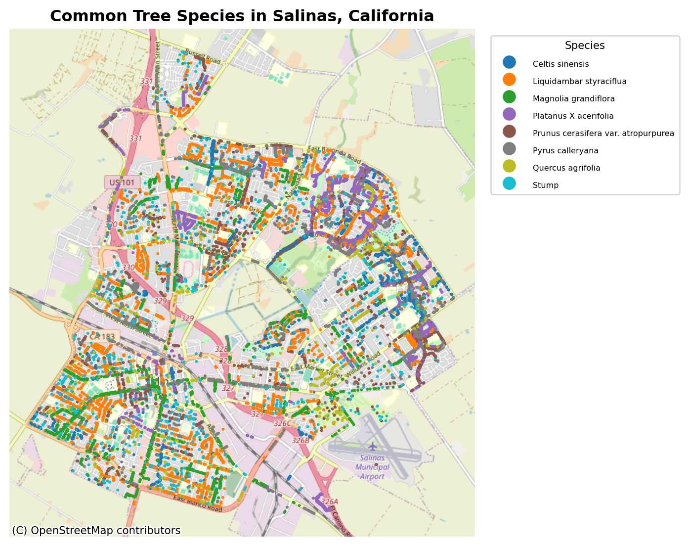

Figure 4: Common tree species, Liquidambar styraciflua and Pyrus calleryana are the most common species

Here, Figure 4 shows the species that dominate the city’s streets.

Tree Sizes and Dimensions

Let’s explore the height and width of the inventory data. First, we will remove trees with missing height and width category. Next, we will categorized the trees into size classes using their DBH:

• Small: DBH < 20 cm
• Medium: 20–40 cm
• Large: 40–60 cm

trees_with_dim = common_trees.dropna(subset=["height","width"])

trees_with_dim["tree_class"] = pd.cut(
    trees_with_dim["dbh"], 
    bins=[0, 20, 40, 60], 
    labels=["small","medium","large"]
)

Visualizing the tree size categories gives a clear picture of the structural diversity:

ax = trees_with_dim.plot(
    column="tree_class", 
    categorical=True, 
    cmap="viridis", 
    legend=True, alpha=0.8,
    markersize = 5
)
cx.add_basemap(ax, source=cx.providers.OpenTopoMap)
plt.axis("off")
legend = ax.get_legend()
legend.set_title("Tree DBH Class", prop={"size": 9})
for text in legend.get_texts():
    text.set_fontsize(6)
legend.get_frame().set_alpha(.8)
legend.set_bbox_to_anchor((1.02, 1))
legend.set_loc("upper right")
plt.title(
    "Tree Sizes in Salinas, California", 
    fontsize=10, 
    fontweight="bold"
)
plt.tight_layout()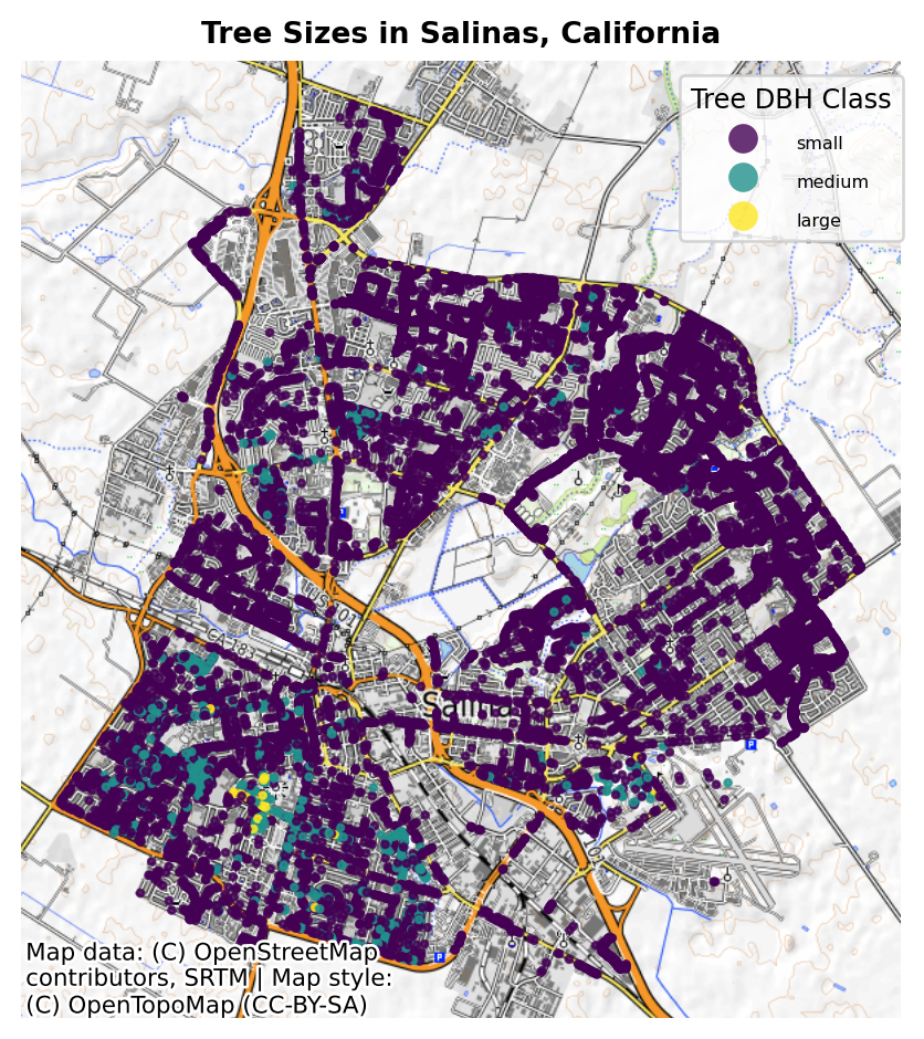

Figure 5: Tree Size Category

Health Condition of the Trees

Let’s explore the health condition of the trees.

common_trees.explore(
    column="cond",
    categorical=True
)

Make this Notebook Trusted to load map: File -> Trust Notebook

Figure 6: Tree chealth conditions

Most of the trees are in a fair to good health state.

Key Takeaways 🌱

Salinas’ tree inventory contains thousands of mapped trees, each with attributes like species, size, and condition. Visualization reveals both species distribution and structural variation across the city.

Categorizing trees into size classes highlights urban forestry trends that could inform management, replacement, and planting decisions. By combining open data with Python’s geospatial stack, we can turn raw tree inventories into insights for greener, healthier cities.