# R Code
install.packages("reticulate")A Short Introduction
I saw an interesting blog post by Nicole Renner on combining R and Python in a Quarto document and I decided to replicate that. Quarto has been seen as the next generation of RMarkdown with support for multiple languages. In this blog post we will interchangeably use the R and Python for a simple EDA on the Palmer penguins dataset. To ensure easy interchange between both languages, we will use the reticulate package by Thomasz Kalinowski, Kevin Ushey, J. J. Allaire, and Yuan Tang.
The Reticulate Package
The reticulate package provides a set of tool for the coordination between python and R. This means that it allows python to be used interactively within an R session. This is beautiful, because the strength of both packages can be utilized to the fullest. To know more about the reticulate package the documentation.
Initial Set Up
The version of R used is R version 4.4.2 (2024-10-31) and RStudio is Cranberry Hibiscus Release (c8fc7aee, 2024-09-16) for Ubuntu Jammy. To ensure interoperability between R and Python there are some things we need to put in place. First, we need to ensure that python is properly configured to work in R studio. On the menus click on Tools > Global Options > Python > find interpreter and choose a python version of your choice. Next we have to install the reticulate package. Entering the command below to install reticulate
After that, load the package into your current session and that is it. The other R packages to be used for this project in R will also be loaded at once.
# R Code
library(reticulate)
library(tidyverse)
── Attaching core tidyverse packages ──────────────────────── tidyverse 2.0.0 ──
✔ dplyr 1.1.4 ✔ readr 2.1.5
✔ forcats 1.0.0 ✔ stringr 1.5.1
✔ ggplot2 3.5.1 ✔ tibble 3.2.1
✔ lubridate 1.9.4 ✔ tidyr 1.3.1
✔ purrr 1.0.4
── Conflicts ────────────────────────────────────────── tidyverse_conflicts() ──
✖ dplyr::filter() masks stats::filter()
✖ dplyr::lag() masks stats::lag()
ℹ Use the conflicted package (<http://conflicted.r-lib.org/>) to force all conflicts to become errorslibrary(ggthemes)
library(latex2exp)We can use the pip to also install necessary packages we’ll be needing.
# Python Code
!pip install pandas numpy
The above code which is not evaluated/executed would install numpy and pandas.
# Python Code
import pandas as pd
On running the above command, reticulate will call the repl_python() function which makes us interact with python in rstudio. This switches the rstudio console from > of R to >>> of python. Seeing these symbols indicates that we can execute python commands. To return to R you can enter exit or quit in the console, but you probably won’t want to exit and restart python interpreter. I’ll show a better way to use both program(R and Python) and using them with quarto seems to make them work seamlessly. ## EDA on Palmer Penguins
The approach to this post will be direct Python will be used for data importation and summaries and R for visualization. I’m using R for visualization because in my opinion it possesses the best visualization library. The palmerpenguins data is saved as a csv file and we’ll start with a python code to read the data.
# Python Code
penguins = pd.read_csv("data/penguins")
Next we check the basic characteristics of the data.
# Python Code
penguins.info()
<class 'pandas.core.frame.DataFrame'>
RangeIndex: 344 entries, 0 to 343
Data columns (total 9 columns):
# Column Non-Null Count Dtype
--- ------ -------------- -----
0 Unnamed: 0 344 non-null int64
1 species 344 non-null object
2 island 344 non-null object
3 bill_length_mm 342 non-null float64
4 bill_depth_mm 342 non-null float64
5 flipper_length_mm 342 non-null float64
6 body_mass_g 342 non-null float64
7 sex 333 non-null object
8 year 344 non-null int64
dtypes: float64(4), int64(2), object(3)
memory usage: 24.3+ KBThe Unnamed column is not needed and will be dropped.
# Python Code
penguins_norm = penguins.drop("Unnamed: 0", axis=1)
We can check to see the column names
# Python Code
penguins_norm.columns
Index(['species', 'island', 'bill_length_mm', 'bill_depth_mm',
'flipper_length_mm', 'body_mass_g', 'sex', 'year'],
dtype='object')Next let’s investigate the data for missingness
# Python Code
penguins_norm.isna().sum()
species 0
island 0
bill_length_mm 2
bill_depth_mm 2
flipper_length_mm 2
body_mass_g 2
sex 11
year 0
dtype: int64Some of the columns such as sex, flipper_length_mm, and body_mass_g among others are having missing values. We can remove this and proceed with the analysis.
# Python Code
penguins_clean = penguins_norm.dropna()
penguins_clean.isna().sum()
species 0
island 0
bill_length_mm 0
bill_depth_mm 0
flipper_length_mm 0
body_mass_g 0
sex 0
year 0
dtype: int64We can easily get a good description of the data.
# Python Code
penguins_clean.describe()
bill_length_mm bill_depth_mm ... body_mass_g year
count 333.000000 333.000000 ... 333.000000 333.000000
mean 43.992793 17.164865 ... 4207.057057 2008.042042
std 5.468668 1.969235 ... 805.215802 0.812944
min 32.100000 13.100000 ... 2700.000000 2007.000000
25% 39.500000 15.600000 ... 3550.000000 2007.000000
50% 44.500000 17.300000 ... 4050.000000 2008.000000
75% 48.600000 18.700000 ... 4775.000000 2009.000000
max 59.600000 21.500000 ... 6300.000000 2009.000000
[8 rows x 5 columns]This has worked sweetly so far for python. Just to let us know we can replicate the processes above using R. We can do this by interacting with the python main module using the reticulate object py. This helps us interacts with all python objects created so. The syntax is straightforward. We use the $ with py to access the object of interest in Python’s session.
# R Code

penguins_r <- py$penguins |>
  select(-`Unnamed: 0`) |>
  drop_na()

head(penguins_r)
species island bill_length_mm bill_depth_mm flipper_length_mm body_mass_g
1 Adelie Torgersen 39.1 18.7 181 3750
2 Adelie Torgersen 39.5 17.4 186 3800
3 Adelie Torgersen 40.3 18.0 195 3250
4 Adelie Torgersen 36.7 19.3 193 3450
5 Adelie Torgersen 39.3 20.6 190 3650
6 Adelie Torgersen 38.9 17.8 181 3625
sex year
1 male 2007
2 female 2007
3 female 2007
4 female 2007
5 male 2007
6 female 2007Just like py, we have r to access objects of R session within python. Instead of using $, the dot, (.) is used instead. penguins_r is the same as penguins_clean. We will do some quick summaries using the penguins_r to show how we get R objects into python sessions
# Python Code

penguins_cleaned = r.penguins_r
penguins_cleaned.head()
species island bill_length_mm ... body_mass_g sex year
0 Adelie Torgersen 39.1 ... 3750.0 male 2007.0
1 Adelie Torgersen 39.5 ... 3800.0 female 2007.0
2 Adelie Torgersen 40.3 ... 3250.0 female 2007.0
3 Adelie Torgersen 36.7 ... 3450.0 female 2007.0
4 Adelie Torgersen 39.3 ... 3650.0 male 2007.0
[5 rows x 8 columns]A good start to our analysis would be to count the total number of penguins according to species, then according to their sex
# Python Code
penguins_cleaned.groupby(["species", "sex"]).count()
island bill_length_mm ... body_mass_g year
species sex ...
Adelie female 73 73 ... 73 73
male 73 73 ... 73 73
Chinstrap female 34 34 ... 34 34
male 34 34 ... 34 34
Gentoo female 58 58 ... 58 58
male 61 61 ... 61 61
[6 rows x 6 columns]Now let’s make quick summaries using the data. But first we’ll get all numeric data variable.
# Python Code
numeric_var = penguins_cleaned.loc[:, penguins_cleaned.dtypes == "float64"].columns
numeric_var = numeric_var.drop("year")
numeric_var
Index(['bill_length_mm', 'bill_depth_mm', 'flipper_length_mm', 'body_mass_g'], dtype='object')Using this, we can make good summaries.
Average body mass, bill length, bill depth, and flipper length of penguins according to species and their sexes.
# Python Code
penguins_cleaned.groupby(["species", "sex"])[numeric_var].aggregate("mean").round(1)
bill_length_mm bill_depth_mm flipper_length_mm body_mass_g
species sex
Adelie female 37.3 17.6 187.8 3368.8
male 40.4 19.1 192.4 4043.5
Chinstrap female 46.6 17.6 191.7 3527.2
male 51.1 19.3 199.9 3939.0
Gentoo female 45.6 14.2 212.7 4679.7
male 49.5 15.7 221.5 5484.8It seems male generally have higher body mass, flipper length, bill length and depth than females for each species. It would be interesting to see if there’s a significant difference in the variables between these species and sexes.
We can also make a pivot table of these metrics according and include the island.
# Python Code
penguins_cleaned.pivot_table(values=numeric_var, index="island", columns=["species", "sex"], aggfunc=["mean", "std"], fill_value=0).round(1).unstack()
species sex island
mean bill_depth_mm Adelie female Biscoe 17.7
Dream 17.6
Torgersen 17.6
male Biscoe 19.0
Dream 18.8
...
std flipper_length_mm Gentoo female Dream 0.0
Torgersen 0.0
male Biscoe 5.7
Dream 0.0
Torgersen 0.0
Length: 144, dtype: float64Given all that’s done we can start visualizing the data. First we get our data from the python environment.
# R Code
penguins_tbl <- py$penguins_cleaned
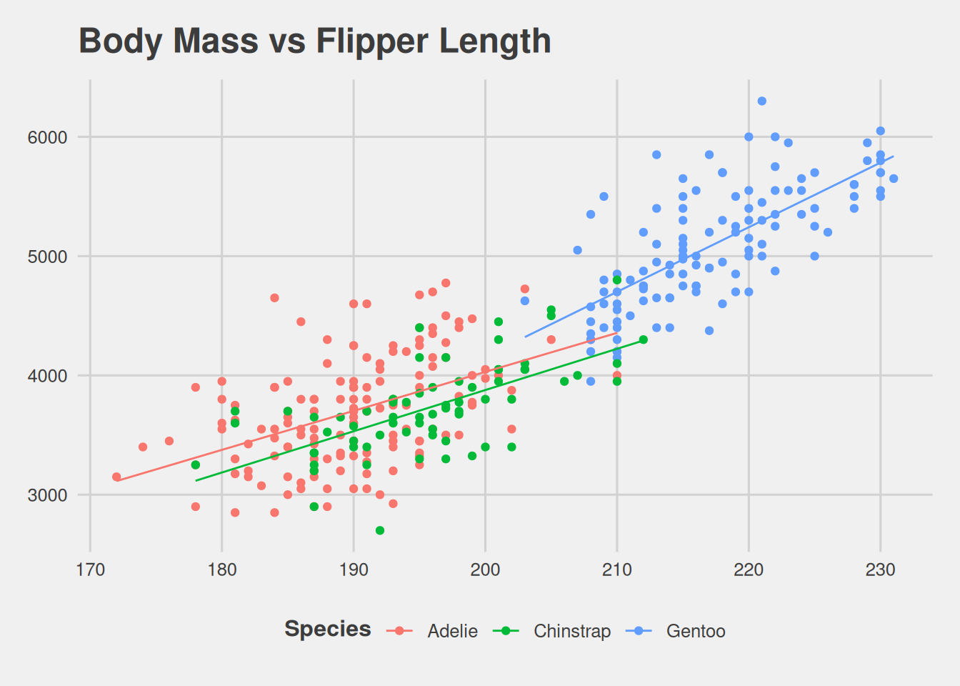
Body Mass vs Flipper Length
# R Code
ggplot(penguins_tbl, aes(flipper_length_mm, body_mass_g, col = species)) +
  geom_point() +
  geom_smooth(
    method = "lm",
    se = FALSE,
    linewidth = .5
  ) +
  scale_fill_colorblind() +
  labs(
    x = TeX(r"(Flipper Length ($mm$))"),
    y = TeX(r"(Body Mass ($g$))"),
    title = TeX("Body Mass vs Flipper Length", bold = TRUE),
    col = TeX("Species", bold = TRUE)
  ) +
  theme_fivethirtyeight()
`geom_smooth()` using formula = 'y ~ x'
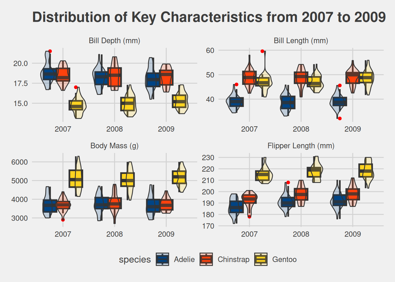
Key Metrics Distribution
# R Code

penguins_long <- penguins_tbl |>
  pivot_longer(
    cols = bill_length_mm:body_mass_g
  ) |>
  mutate(
    name = str_replace_all(name, "_", " "),
    name = str_to_title(name),
    name = str_replace_all(name, "Mm", "(mm)"),
    name = str_replace(name, "G", "(g)")
  )

penguins_long |>
  ggplot(aes(factor(year), value, fill = species)) +
  geom_boxplot(
    position = "dodge",
    outlier.colour = "red",
    linewidth = 1
  ) +
  geom_violin(
    position = "dodge",
    alpha = .2
  ) +
  facet_wrap(~name, scales = "free") +
  labs(
    x = "Year",
    title = TeX(r"(\textbf{Distribution of Key Characteristics from 2007 to 2009})")
  ) +
  scale_fill_calc() +
theme_fivethirtyeight() 
Conclusion
This project highlights one of the strength of using quarto and RMarkdown, and that’s their compatibility with other languages. Here, I used both R and Python in the same project and switched the use of both languages. This is possible using the reticulate package in R, and there’s a similar package to allow easy integration of R in python with the rpy2 package.