# A tibble: 246 × 14
   day   month year  temperature rh    ws    rain  ffmc  dmc   dc    isi   bui
   <chr> <chr> <chr> <chr>       <chr> <chr> <chr> <chr> <chr> <chr> <chr> <chr>
 1 01    06    2012  29          57    18    0     65.7  3.4   7.6   1.3   3.4
 2 02    06    2012  29          61    13    1.3   64.4  4.1   7.6   1     3.9
 3 03    06    2012  26          82    22    13.1  47.1  2.5   7.1   0.3   2.7
 4 04    06    2012  25          89    13    2.5   28.6  1.3   6.9   0     1.7
 5 05    06    2012  27          77    16    0     64.8  3     14.2  1.2   3.9
 6 06    06    2012  31          67    14    0     82.6  5.8   22.2  3.1   7
 7 07    06    2012  33          54    13    0     88.2  9.9   30.5  6.4   10.9
 8 08    06    2012  30          73    15    0     86.6  12.1  38.3  5.6   13.5
 9 09    06    2012  25          88    13    0.2   52.9  7.9   38.8  0.4   10.5
10 10    06    2012  28          79    12    0     73.2  9.5   46.3  1.3   12.6
# ℹ 236 more rows
# ℹ 2 more variables: fwi <chr>, classes <chr>Statistical Analysis of Environmental Data
CIFAG Webinar
2026-04-11
About me
- Founder, EU StudyAssist
- Data scientist
- Educator

How I Got Here
- 2014-2019: Bachelors - Forestry
- 2020-2021 : Teaching Assistant
- 2021-2023: MSc. Forestry
- 2023-: Data Science Consultancy
- 2024-: EU StudyAssist

Important
Visit www.eustudyassist.com to know more about EU StudyAssist
What Is This Talk About?
In this talk we will …
- go through the typical life cycle of environmental data.
- do some data exploration for environmental data, check trends, relationship and more.
- model relationships with Linear Regression.
- diagnose model reliability.

Important
While R is used in this talk, the focus is not just on the statistical tool or a single technique.
Environmental Data Characteristics
Environmental datasets are unique and often challenging:
- Expensive to acquire: inventory data; crop measurements
- Missing Data: Sensors fail; weather happens; inaccessible!
- Measurement Bias: Different instruments, different results.
- Temporal Dependence: Observations can be time-series (e.g., daily sensor data).
- Spatial Autocorrelation: Sites closer together tend to share similar properties.

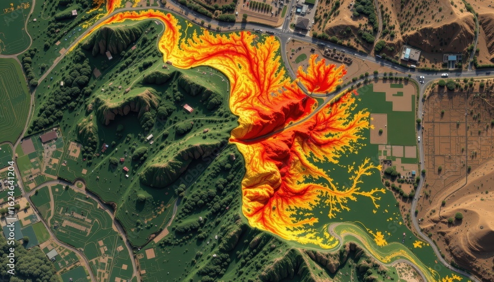
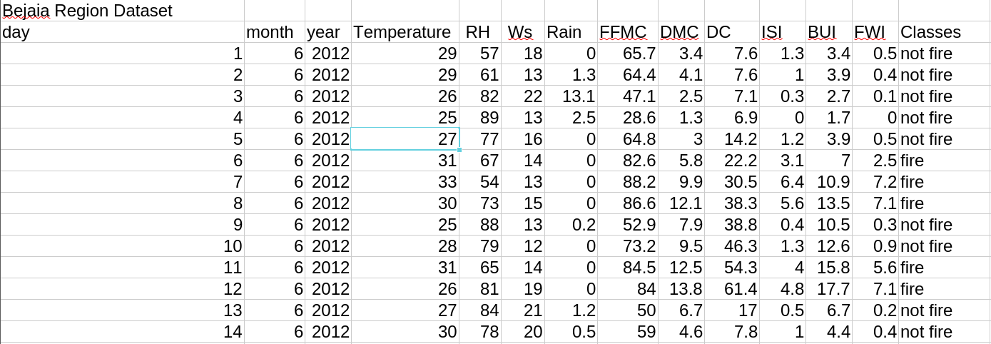
The Data
- Algeria wildfire dataset.
- Occurrence of wild fire
- Estimate the danger of wildfire occurring.
variables of interest
- occurrence of a wildfire during the summer (fire/no fire)
- FWI of forest
Note
Forest Weather Index (FWI) is a global index that estimates wildfire danger by calculating fuel moisture and fire behavior based on temperature, relative humidity, wind speed, and precipitation.
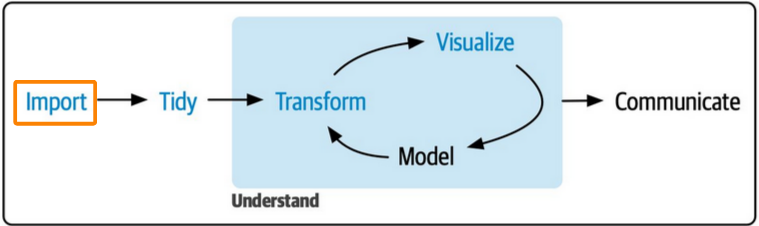
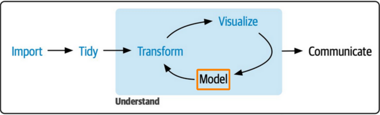
Data Science/Analysis Workflow
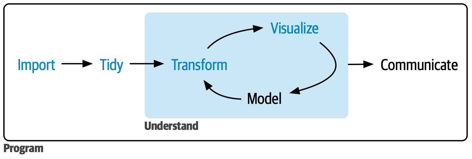
STEP I: Data Import
Exploratory Data Analysis (EDA)
- Cleaning: Handling missing values; unit conversions; general cleaning.
- Transformation: filtering data, summarizing, and working on data as a group.
- Visualization: Trends, distributions, and outliers.
- Correlation: Do variables move together?
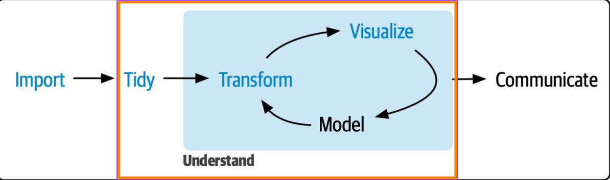
Data exploration is a thorough repetitive process
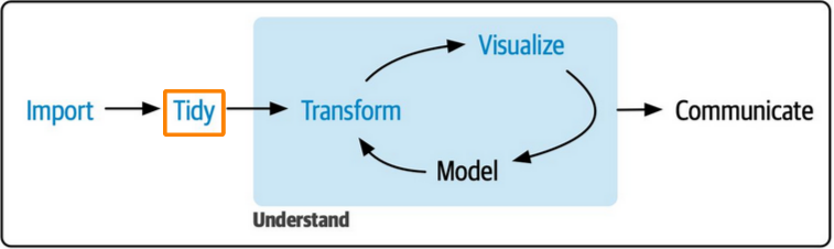
STEP II: Tidy
- Confirm property of your data
- Get quick summary of data
- Try to identify discrepancies in your data
- Remove or impute rows
- Ensure variables have the right data types
- Check for outliers
STEP III: Transform
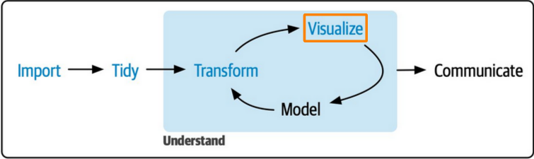
STEP IV: Visualize
A working plan
- focus on variables of interest first
- focus on other variables next
- visualize relationships between variables
STEP IV: Visualize …
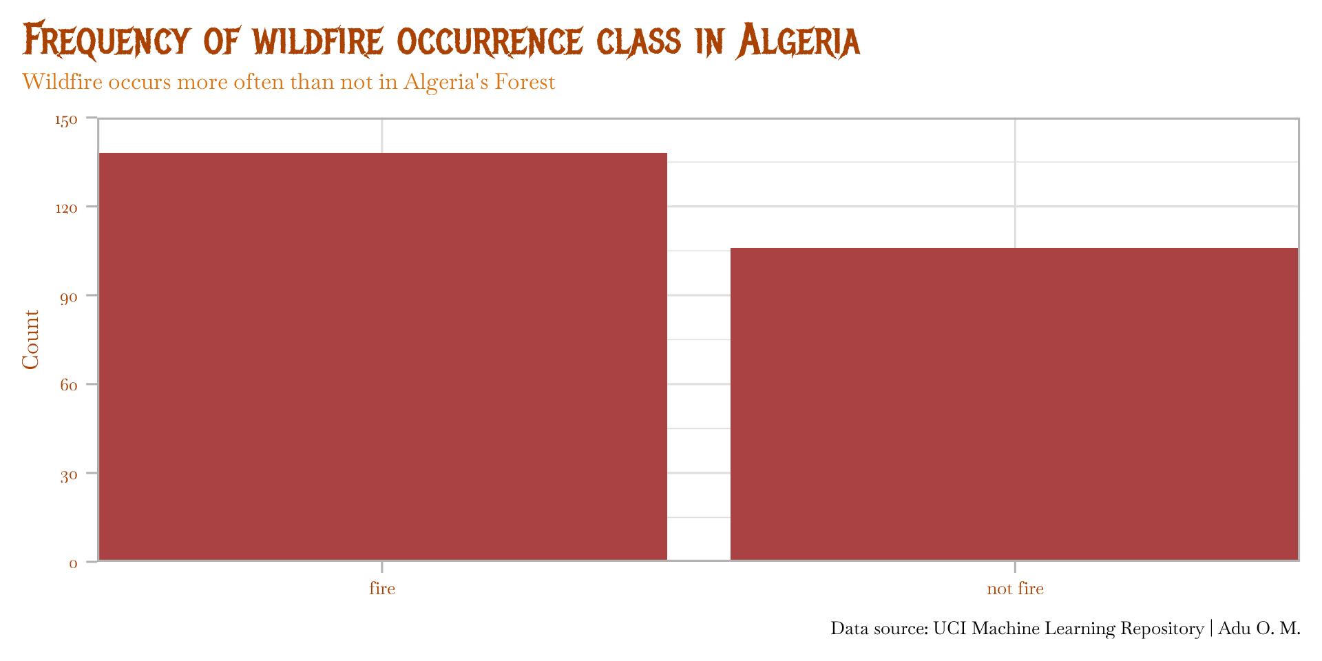
Response variable (fire occurrence)
- Univariate plot
- Categorical data
Code
algeria_tbl |>
  ggplot(aes(classes))  +
  geom_bar(fill = "#AA4243") +
  labs(
    y = "Count",
    title = "Frequency of wildfire occurrence class in Algeria",
    subtitle = "Wildfire occurs more often than not in Algeria's Forest",
    caption = "Data source: UCI Machine Learning Repository | Adu O. M."
  ) +
  scale_y_continuous(
    breaks = seq(0, 150, 30),
    limits = c(0, 150)
  ) +
  theme_light(
    base_size = 24,
    base_family = "bsk"
  ) +
  coord_cartesian(expand = FALSE) +
  theme(
    plot.title.position = "plot",
    plot.title = element_text(
      colour = "#AA4203",
      family = title_font,
      size = 48,
      margin = margin(b = 5, unit = "pt")
    ),
    axis.title.x = element_blank(),
    plot.subtitle = element_text(color = "#dc730e"),
    axis.text = element_text(color = "#AA4203"),
    axis.title.y = element_text(color = "#AA4203")
  )
STEP IV: Visualize …
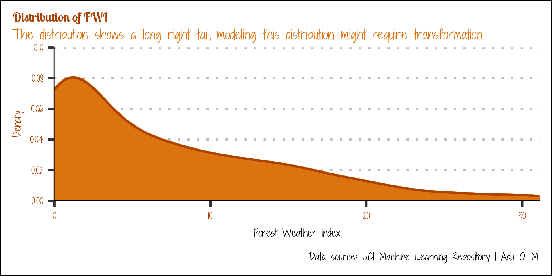
Response Variable (FWI)
- Univariate plot
- Continuous data
Code
algeria_tbl |>
ggplot(aes(fwi)) +
geom_histogram(
stat = "density",
col = "#dc730e"
) +
geom_density(
linewidth = 1.3,
col = "#AA4203"
) +
theme_clean(
base_size = 32,
base_family = main_font_2
) +
scale_y_continuous(
breaks = seq(0, .1, .02),
limits = c(0, .1)
) +
labs(
x = "Forest Weather Index",
y = "Density",
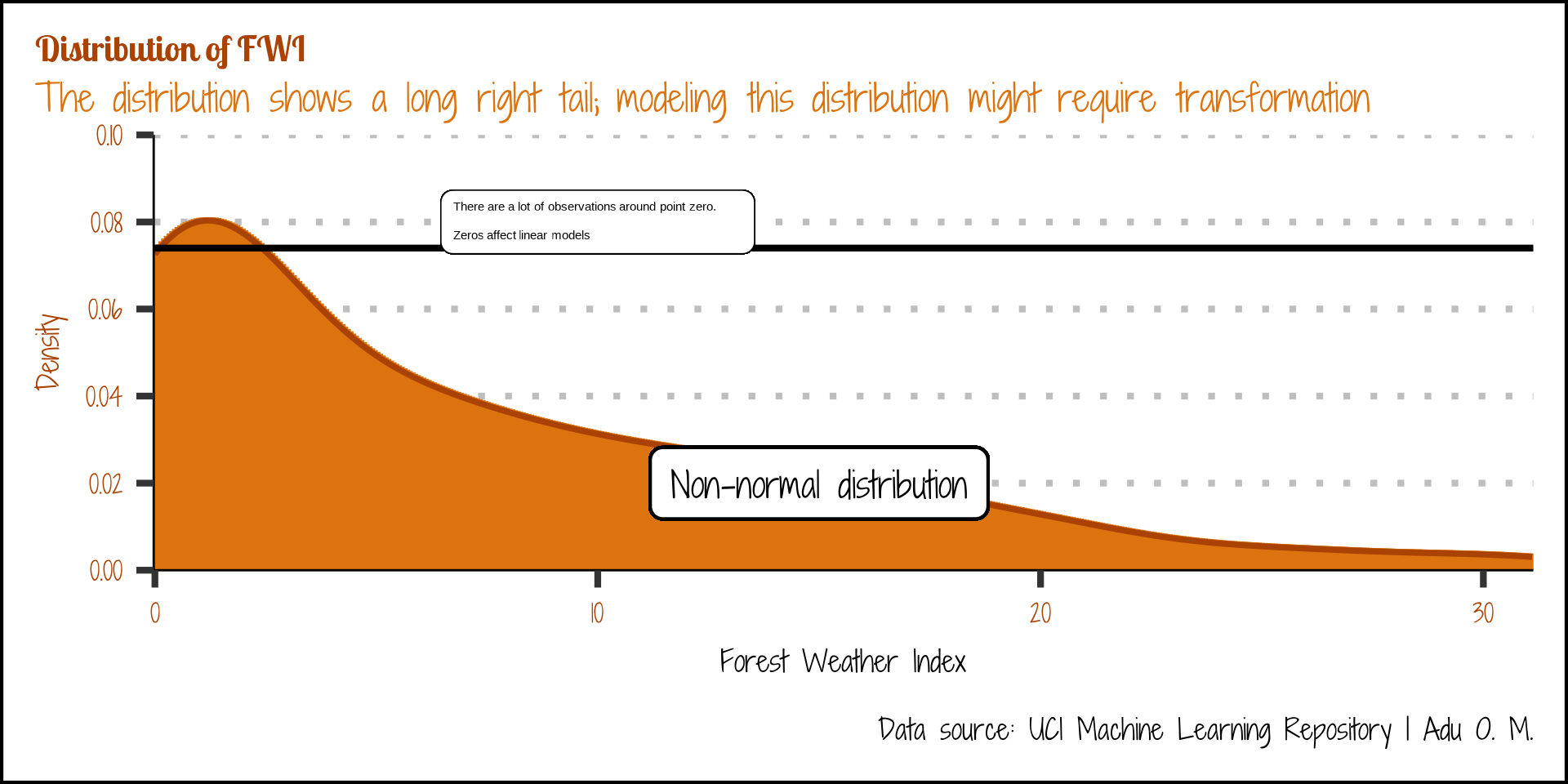
title = "Distribution of FWI",
subtitle = "The distribution shows a long right tail; modeling this distribution might require transformation",
caption = "Data source: UCI Machine Learning Repository | Adu O. M."
) +
coord_cartesian(expand = FALSE) +
theme(
plot.title.position = "plot",
plot.title = element_text(
colour = "#AA4203",
family = title_font_2,
size = 32,
margin = margin(b = 5, unit = "pt")
),
plot.subtitle = element_textbox_simple(
color = "#dc730e",
margin = margin(b = 5, unit = "pt")
),
axis.text = element_text(color = "#AA4203"),
axis.title.y = element_text(color = "#AA4203")
)
STEP IV: Visualize …
Explanatory Variable
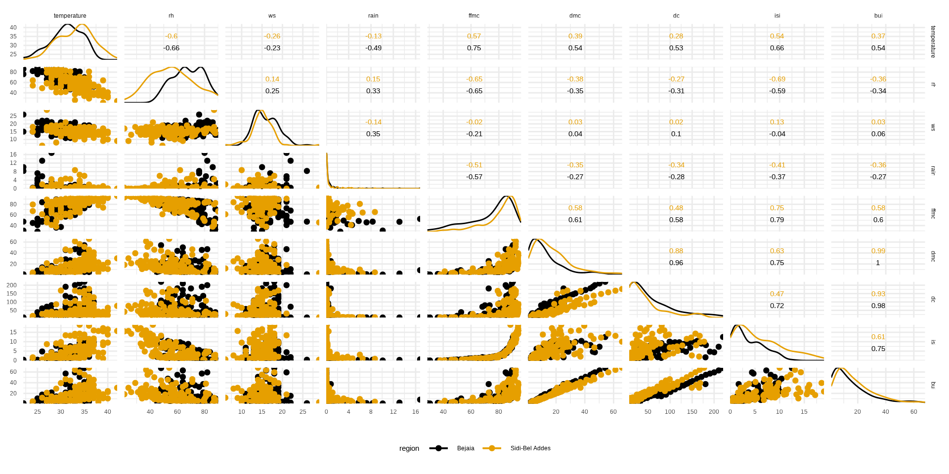
STEP IV Visualize …
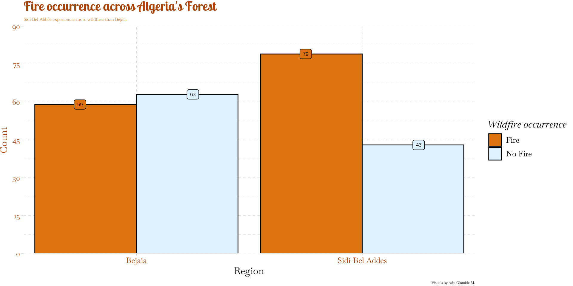
Response vs explanatory variable
- Bivariate plot
- Categorical vs Categorical data
Code
algeria_tbl |>
  summarize(
    .by = c(region, classes),
    count = n()
  ) |>
  ggplot(aes(region, count, fill = classes)) +
  geom_col(position = "dodge", col = "#030303") +
  labs(
    x = "Region",
    y = "Count",
    fill = "Wildfire occurrence",
    title = "Fire occurrence across Algeria's Forest",
    subtitle = "Sidi Bel Abbès experiences more wildfires than Béjaïa",
    caption = "Visuals by Adu Olamide M."
  ) +
  geom_label(
    aes(label = count),
    position = position_dodge(width = 1),
    show.legend = FALSE,
    size = 4.5
  ) +
  scale_y_continuous(
    limits = c(0, 90),
    breaks = seq(0, 90, 15)
  ) +
  scale_fill_manual(
    values = c("#dc730e", "#dcf3ff"),
    labels = c("Fire", "No Fire")
  ) +
  coord_cartesian(expand = FALSE) +
  theme_pander(
    base_size = 24,
    base_family = main_font
  ) +
  theme(
    plot.title = element_text(
      colour = "#AA4203",
      family = title_font_2,
      size = 32,
      margin = margin(b = 5, unit = "pt")
    ),
    plot.subtitle = element_textbox_simple(
      color = "#dc730e",
      margin = margin(b = 5, unit = "pt")
    ),
    axis.text = element_text(color = "#AA4203"),
    axis.title.y = element_text(color = "#AA4203")
  )
STEP IV: Visualize …
Response vs explanatory variable
- bivariate plot
- Continuous vs continuous
Code
algeria_tbl |>
ggplot(aes(date, fwi,)) +
geom_line(
linewidth = 0.8,
col = "#AA470e"
) +
theme_pander(base_size = 24) +
labs(
x = "Date",
y = "FWI",
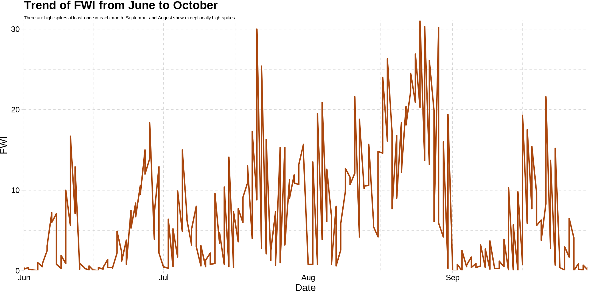
title = "Trend of FWI from June to October",
subtitle = "There are high spikes at least once in each month. September and August show exceptionally high spikes"
) +
coord_cartesian(expand = FALSE) +
theme (
plot.subtitle = element_textbox_simple()
)
STEP IV: Visualize …
Response vs explanatory variable
- multivariate plot
- Categorical vs continuous
Code
algeria_tbl |>
ggplot(aes(date, fwi, col = classes)) +
geom_line() +
facet_wrap(~region)+
theme_pander(
base_size = 24,
base_family = main_font
) +
labs (
y = "FWI",
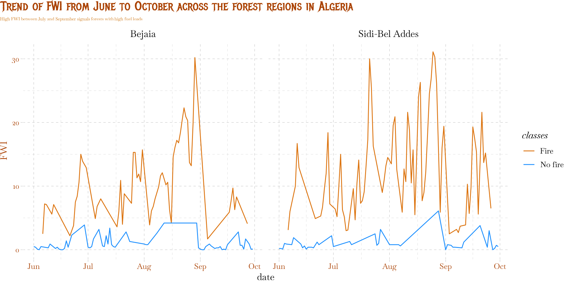
title = "Trend of FWI from June to October across the forest regions in Algeria",
subtitle = "High FWI between July and September signals forests with high fuel loads"
) +
scale_color_manual(
values = c("#dc730e", "dodgerblue"),
label = c("Fire", "No fire")
) +
theme(
plot.title.position = "plot",
plot.title = element_text(
colour = "#AA4203",
family = title_font,
size = 32,
margin = margin(b = 5, unit = "pt")
),
plot.subtitle = element_textbox_simple(
color = "#cd730e",
margin = margin(b = 5, unit = "pt")
),
axis.text = element_text(color = "#AA4203"),
axis.title.y = element_text(color = "#AA4203")
)
Some factors that influence the choice of models
- data types: categorical (binomial, multinomial) / continuous / discrete (count)
- size of data
- linearity of variables
- distribution of variables (normal / non-normal data / tweedie)
- explainability vs prediction
Are the Assumptions Met?
- Linearity: Is the relationship truly a straight line?
- Independence: Are errors related?
- Normality: Are residuals bell-shaped?
- Homoscedasticity: Constant variation?

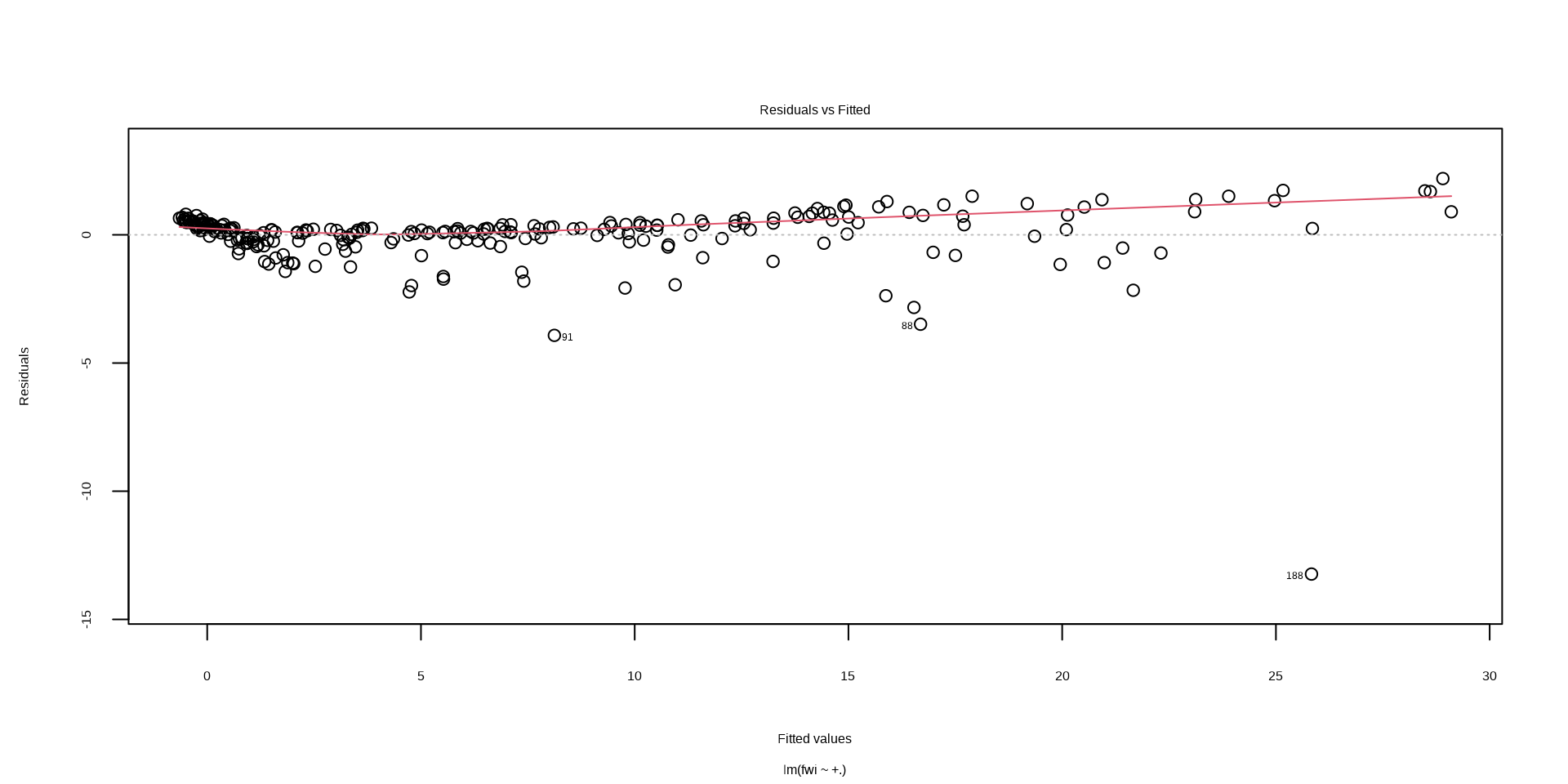
Model Interpretation
While the model captured signals well, it shows:
- heteroscedasticity (fan shape). It captures lower values more accurately than higher values.
- potential non-linear relationship. There is a pattern in the data that the current linear model is missing.
Code
algeria_tbl |>
  ggplot(aes(fwi)) +
  geom_histogram(
    stat = "density",
    col = "#dc730e"
  ) +
  geom_density(
    linewidth = 1.3,
    col = "#AA4203"
  ) +
  geom_label(
    aes(
      x = 15,
      y = 0.02,
      label = "Non-normal distribution")
  ) +
  geom_hline(aes(yintercept = 0.074, x=25)) +
  geom_textbox(
    aes(x = 10, y = 0.08, label = "There are a lot of observations around point zero. Zeros affect linear models")
  ) +
  theme_clean(
    base_size = 32,
    base_family = main_font_2
  ) +
  scale_y_continuous(
    breaks = seq(0, .1, .02),
    limits = c(0, .1)
  ) +
  labs(
    x = "Forest Weather Index",
    y = "Density",
    title = "Distribution of FWI",
    subtitle = "The distribution shows a long right tail; modeling this distribution might require transformation",
    caption = "Data source: UCI Machine Learning Repository | Adu O. M."
  ) +
  coord_cartesian(expand = FALSE) +
  theme(
    plot.title.position = "plot",
    plot.title = element_text(
      colour = "#AA4203",
      family = title_font_2,
      size = 32,
      margin = margin(b = 5, unit = "pt")
    ),
    plot.subtitle = element_textbox_simple(
      color = "#dc730e",
      margin = margin(b = 5, unit = "pt")
    ),
    axis.text = element_text(color = "#AA4203"),
    axis.title.y = element_text(color = "#AA4203")
  )